Excel TAKE Function – How To Use

The TAKE function allows us to extract a subset of ranges or arrays from a bigger dataset. The function is especially useful when dealing with large datasets as it makes data manipulation and extraction easier and faster.

While using the TAKE function, the user can choose the number of rows or columns to be extracted from the beginning or the end of the array.

Syntax

The syntax of the TAKE function consists of three arguments and is structured as follows.

Arguments:

The TAKE function accepts two mandatory arguments while the third is optional. The role of each input argument is stated below.

'array' – This is the first and only mandatory argument of the TAKE function. It accepts the value of the original cell range or array from which we wish to extract the rows or columns. The input value of the array argument can also be a static array or a return value from another function.

'rows' – This is a mandatory argument that indicates the number of rows we wish to extract from the original The argument must be mentioned in the formula (by way of a comma) even if it is left empty. When the value of the rows argument is left empty, the TAKE function returns all the rows from the original array.

Another aspect of the rows argument is if the input value is a positive number, the function retrieves the row(s) from the top of the array. Conversely, when a negative value is given, it extracts row(s) from the bottom of the array.

'cols' – This is an optional argument that accepts the value of the number of columns to be extracted from the input The positive value of the cols argument indicates that the TAKE function will extract the column(s) from the left of the array. Meanwhile, a negative value suggests that column(s) must be extracted from right to left. If the cols argument is left empty, the function returns all the column(s) from the input array.

Important Characteristics of the TAKE Function

One of the basic features of the TAKE function is that it creates a new array containing the specified rows and columns. Furthermore, the TAKE function offers several notable features, outlined below.

• If the value of the rows or cols argument is greater than the input array, the TAKE function returns all the rows or columns of the complete input array.
• If the input array is empty, the TAKE function returns an array of 0s depending on the rows and columns argument.
• When the array argument is left empty, the function throws a #VALUE! error.
• When the rows or cols argument is set to 0, the TAKE function results in a #CALC! error.

With the aforementioned features in consideration, let's move on to comprehending the workings of the TAKE function and how it interacts with data.

Examples of TAKE Function

To better understand the TAKE function in Excel, let's start by using different input values for each argument to demonstrate how it functions and the outcomes it produces. This will help us grasp its mechanics and utility more comprehensively.

Here, we have taken a small dataset that consists of 3 rows and columns.

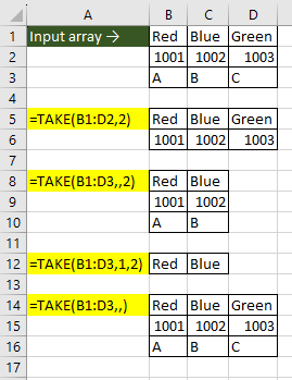
In the first example, only the input value for the first two arguments is used, and the cols argument is left empty. As a result, the TAKE function extracts the first 2 rows from the range B1:D2, while returning all columns.

The next example showcases the same logic but for columns. Here, as observed, we have skipped the input value for the rows argument. As intended, the function extracted all rows and the first 2 columns from the range B1:D3.

The subsequent instance is a classic example where the input values for all arguments are used. The TAKE function considers the number of rows and columns and extracts the first row and 2 columns from the given dataset.

In the last example, as the input values for both the rows and cols arguments are empty, the TAKE function simply returns the entire input range B1:D3 as the output.

Now that the basic functionality of the TAKE function is clear, let's explore more examples to showcase its capabilities to retrieve specific portions of information from larger datasets.

Example 1 – Simple Use of the TAKE Function

Suppose you are organizing a few workshops that have limited seating and follow a first come, first serve enrollment process. Due to its popularity, you have received several applicants which are now stored in an Excel dataset that includes information such as the applicant's names, contact details, workshop preferences, and enrollment timestamps.

After the application period concludes, you intend to extract the first 5 applicants as they are sorted as per enrollment timestamp and notify them about their application status.

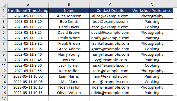
Using the TAKE function, we can easily extract the first 5 applicants and the relevant columns. Subsequently, we can leverage the extracted subset for any further use. The function used will be as follows.

This will extract the first 6 rows from the dataset A1:D16 along with the last 3 columns as we do not need the enrollment timestamps column. We are extracting the first 6 rows which include the row header and the first 5 applicants.

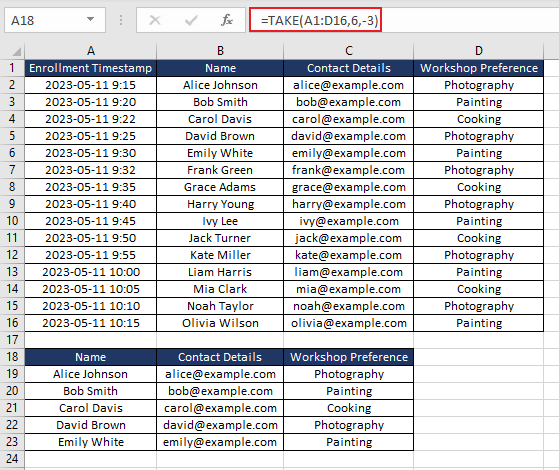
This exemplifies a classic application of the TAKE function. Let's delve deeper to uncover additional scenarios where the same function proves valuable.

Example 2 – Calculating Average of Last N Numbers with TAKE Function

Suppose we wish to analyze the stock prices of a company over a period, and we want to calculate the average closing price of the last N trading days to identify recent price trends. We downloaded the stock price trading data which keeps updating each day.

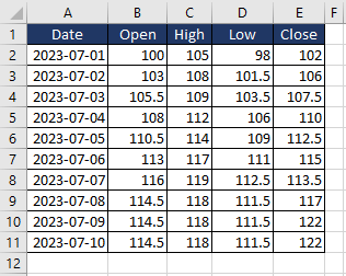
We can use the TAKE function to extract the last N days of data and then use the AVERAGE function to calculate the average. Let's say we wish to calculate the average closing price for the last 5 days. The formula to extract the intended values will be as follows.

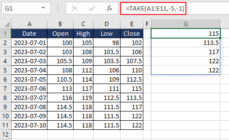
Now we can simply use the AVERAGE function as follows.

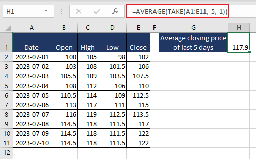
We have obtained the desired average closing price, but it's important to acknowledge a limitation in this approach. With the stock price dataset expanding daily, the formula needs to be adaptable and encompass the newly added rows to remain effective.

There are two ways we can achieve that. One way is to format the existing dataset as a Table in Excel. Select the dataset which is $A$1:$E$11 and press the Ctrl + T shortcut. Alternatively, choose Format as Table option from the Home Tab.

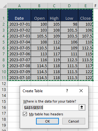
After we press OK, the table is created. Now, to rename the table as per your preference, go to the Table Design tab, select the existing name in the Table Name box, and overwrite it with a new one. We have named it 'stockprice'.

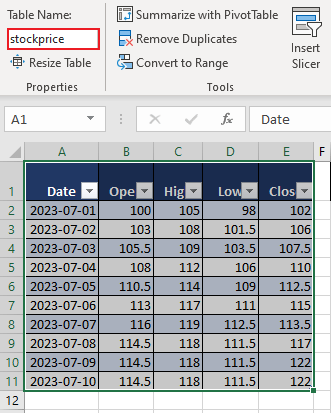
Now the formula used will be as follows.

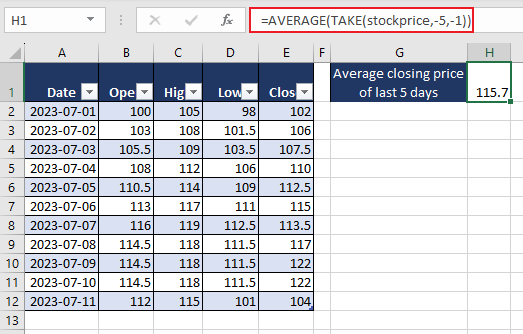
As we can see, an additional row has been added and the formula dynamically encompasses the most recent 5 rows.

Another way to achieve this is by combining the FILTER function with the TAKE function. We can include the entire column E as the input array and FILTER the range of cells that are non-empty. We can then use the TAKE function on the filtered data and extract the last 5 values.

The function will be as follows.

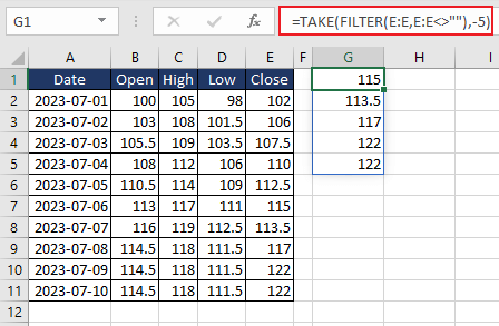
Now, we can easily calculate the average of the filtered data. The formula will be as follows.

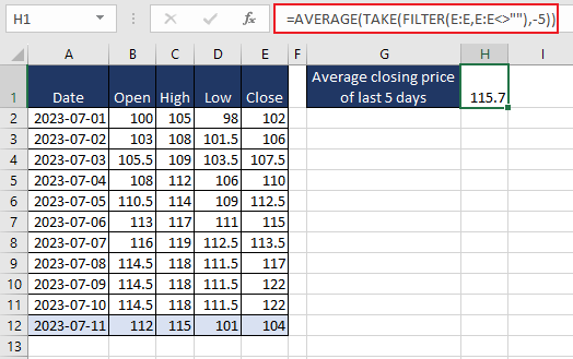
As observed, we now have the average closing price for the last 5 days and the formula remains unaffected even after incorporating an additional row. As a practice, try to use the combination of FILTER and TAKE functions to extract the last day's data when the High price was more than 115.

Example 3 – Using SORTBY and TAKE Function

Suppose you have a dataset containing movie titles, user ratings, release years, and genres. You now wish to extract the highest and lowest-rated movies within different genres from a huge dataset.

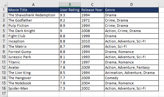
To achieve this, we will begin by sorting the dataset based on user ratings. Subsequently, we will use the TAKE function to extract both the top and bottom movie names.

The following formula will rearrange the "Movie Title" column (A2:A16) based on the corresponding user ratings in the "User Rating" column (B2:B16) in descending order (-1). This means the movies will be arranged from highest to lowest user ratings.

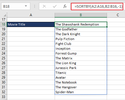
We can now easily extract the first and last movie names from the sorted data indicating the highest and lowest rated. The formula used will be as follows.

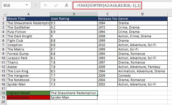
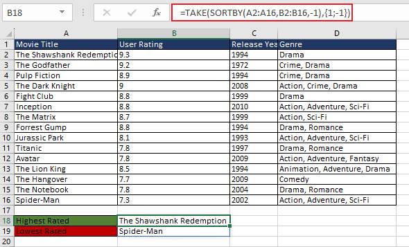
Let's go a step further and get rid of the need to use two different formulas. This can be achieved by using an array as an input for rows. The formula used will be as follows.

The array input {1; -1} tells the TAKE function to extract the first and last row from the sorted array. The semicolon will spill the result vertically.

Example 4 – Using TAKE Function on Separate Datasets

Imagine you own a retail store that sells electronics, clothing, and home goods. You now have sales data for different products under each category, organized in separate datasets. The aim is to identify the top 3 selling products across all categories for a special promotional campaign.

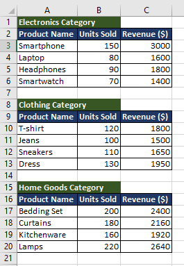
As there are separate datasets for each category, the first step is to use the VSTACK function to vertically combine the three category datasets, creating a merged dataset. The formula used will be as follows.

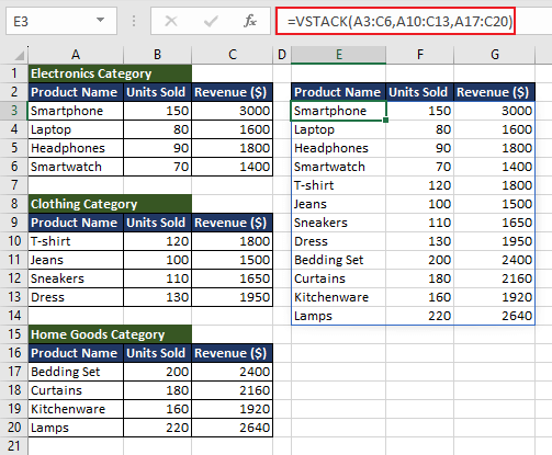
Now, we can reorder the combined dataset using the SORT function based on the Units Sold column (column 2) in descending order (-1). The formula will be as follows.

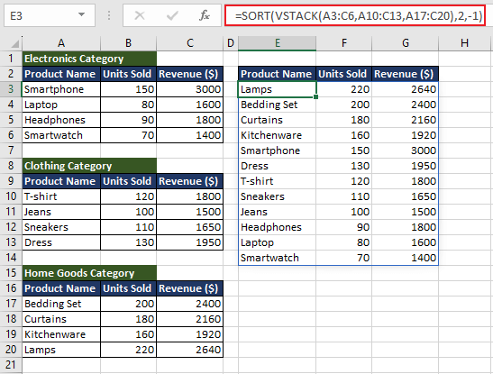
Now, the dataset is sorted in a manner where the product with the highest quantity of units sold is on the top. In the final step, we can use the TAKE function to extract the first 3 rows indicating the top 3 selling products. The final formula will be as follows.

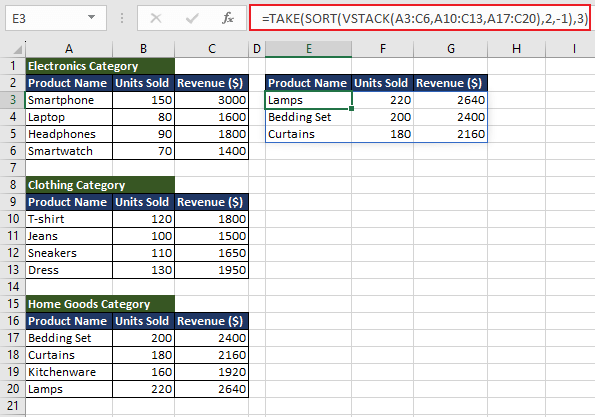
The same logic can be used to combine data from different worksheets or combine them horizontally using HSTACK function and then use the TAKE function to extract the desired data.

TAKE Function vs DROP Function

Suppose you have a dataset related to soccer league standings of various teams. The data includes details such as team name, matches played, number of wins, draws, losses, and the points earned by each team. The aim is to extract the top 5 teams in the standings and remove the last 5 teams.

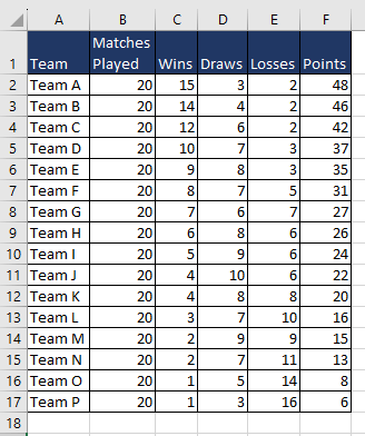
As we already know, the TAKE function can be used to extract the required rows and columns. Therefore, we can use the TAKE function to extract the top 5 rows representing the top teams. The formula used will be as follows.

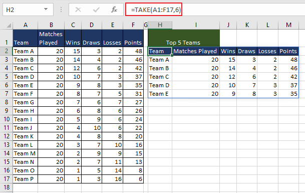
On the contrary, the DROP function can be used to remove the required rows and columns. So, we can utilize the DROP function in this case and remove the last 5 teams which have the minimum points. The function used will be as follows.

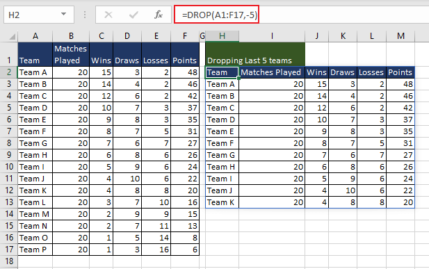
The function, therefore, excluded the last five rows indicated by the negative input value.

Both the TAKE and DROP functions showcase complementary features used in data manipulation in Excel where in both cases we can extract a subset from a larger data. One function retains the data while the other removes it.

The TAKE function helps us retrieve the desired rows and columns, yet its constraint lies in its exclusive extraction of neighboring rows and columns. To extract non-adjacent rows or columns, we can use the CHOOSEROWS function or CHOOSECOLS function.

Delve deeper into the manifold applications of the TAKE function and unlock its versatile potential to elevate both your Excel proficiency and data analysis skills. Meanwhile, we bring to you yet another Excel function to expand your repertoire of tools and techniques.