How to Format Phone Number in Excel (3 Quick Ways)

If you see this number in Excel: 9876543210

Would it register to you as a phone number? Not to us either. What makes a phone number look like a phone number? Some characteristic hyphens and parentheses would be a great deal helpful.

Let’s have a look at how it would change things: (987)654-3210

Definitely rings right! (See what we did there?)

Evidently, it’s all in the formatting. In this tutorial, you will find how to format phone numbers in Excel. We will see how to use Excel's built-in phone number formats, a custom format, and the TEXT function, and how to deal with phone numbers starting with 0.

We need an example to explain all of this so, here it comes.

Example

We will show you how to format phone numbers using the example below:

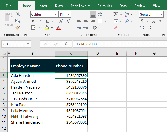
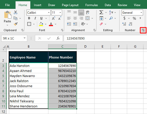
We have a collection of phone numbers in column C, all of which are 10-digit numbers. This is of course a dummy example with no real phone number. Our target today is to format these numbers because as of now, they don’t look like phone numbers, do they?

To be formatted as phone numbers, some of the methods below (mentioned with Pro Tip) require the numbers to be entered as plain numbers with the default General number format, as shown in this example. We can now proceed with our attempts at making these numbers look like phone numbers.

Let’s get formatting!

Method #1 – Using Built-in Excel Format

Let’s start with a built-in format in Excel to format numbers as phone numbers. The cell formatting options in Excel have a Special setting to format phone numbers according to the location. The layout of a phone number may differ in number of digits and/or the signs used in the number e.g. where the parentheses and hyphens are placed. Selected from the options, a country’s phone number format can be applied to numbers. The steps to do this are as follows:

Pro Tip: Make sure the numbers that you want to format are in the default number format i.e. General and are devoid of any characters and signs. If this is not the case, the format will not apply on the numbers.

• Select the numbers for formatting.
• Click on the dialog box launcher of the Number group in the Home tab or press the Ctrl + 1 keys to open the Format Cells dialog box.
• 
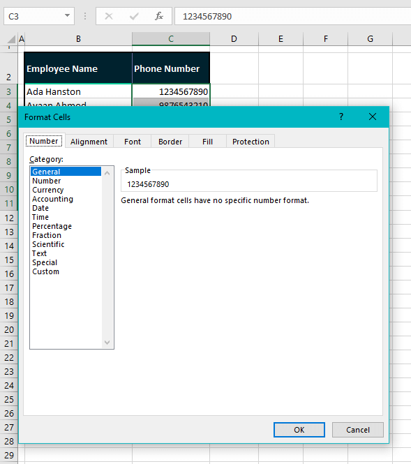
• If all the selected cells are in the General Number format, the dialog box will open with the General category selected:
• 
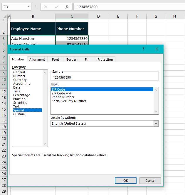
• Select Special from the left Category. The first Locale that will appear by default is English (United States). For the purpose of this tutorial, we’ll go ahead with this.
• 
• Select a Locale from the given list.
• Excel may or may not have a phone number format for the selected locale.
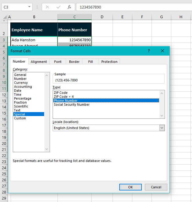
• If available for the selected Locale, click on Phone Number from the Type
• You can see the preview in the Sample field:
• 
• Click on the OK command button when done.

The selected numbers will be formatted as phone numbers as per the selected Special format, which is shown in the Number Format box:

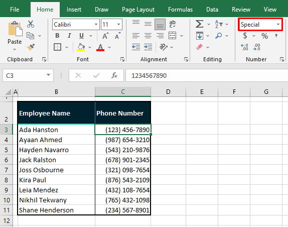
Note that this only changes the display of the numbers. The value of the formatted cell can be seen in the Formula Bar and is, basically, a numeric value that has been formatted.

If the preset formats aren’t doing it for you, there’s an option to create a custom format. Good idea? Let’s talk about it then.

Method #2 – Using Custom Format

If you haven't found a preset format up to your requirement, you can set up a custom format by a formatting code to display numbers as phone numbers. Again, we will be using the Format Cells settings to apply a custom format to the numbers. The following are the steps to format phone numbers using Custom format:

Pro Tip: For an idea of how the code works, you can select a Locale in the Special category and then head to the Custom category to format the code as a starting base.

• Select the range with the numbers.
• Open the Format Cells dialog box by pressing Ctrl +1 or using the dialog box launcher in the Home tab’s Number
• 
• From the left pane, select Custom from the Category
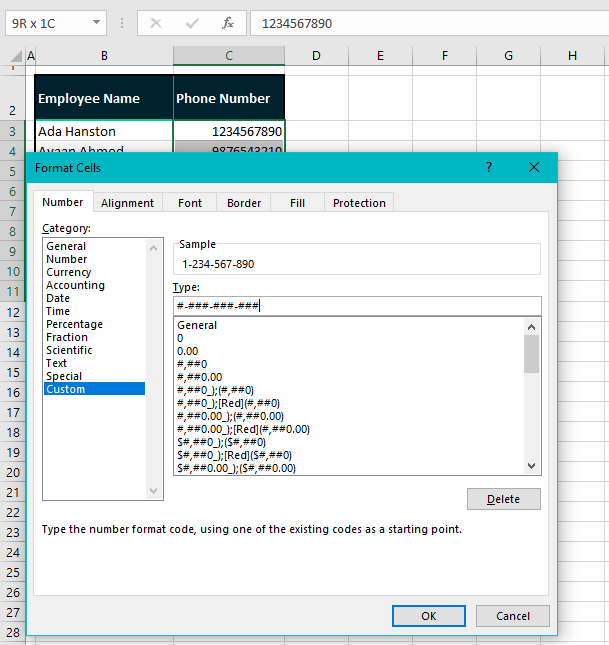
• Enter a formatting code in the Type field e.g. we want every 3 digits from the end hyphenated so here’s the code we will enter:
• #-###-###-###
  
• Then select the OK

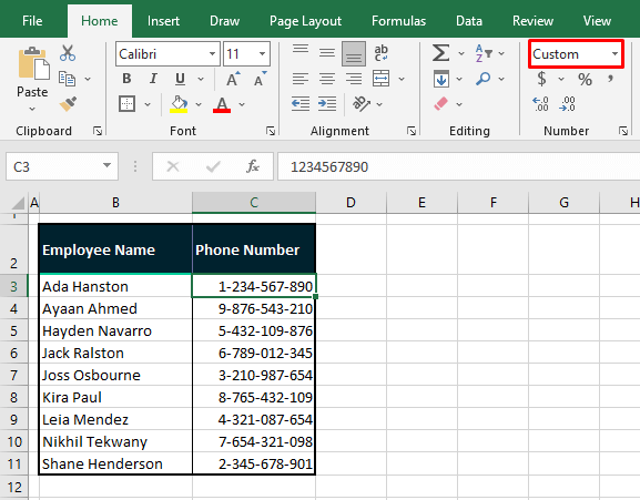
The numbers in selection will be formatted according to the set Custom Format:

Note: Custom formats apply only to the current workbook and must be recreated to be used in another workbook.

Method #3 – Using TEXT Function

To format phone numbers in Excel, we can use the TEXT function. The TEXT function converts a value to text in the specific provided format. It is to be noted however that the value will be converted into text and therefore cannot be used in calculations and number functions. Let’s see a couple of ways we can involve the TEXT function to format phone numbers.

Pro Tip: Clear the number of any signs and other characters and make sure the numbers are in the General Number format before you use the TEXT function.

TEXT function with Same Digit Numbers

Firstly, we'll use the function with 10-digit numbers which means that we'll use one function for numbers that all bear the same number of digits. Below is the formula using the TEXT function to format phone numbers:

The TEXT function takes the value in cell C3. Let's say we want the area code of the phone number to be enclosed in parentheses and then a hyphen after the first 3 digits. This is the format we will supply to the TEXT function for conversion of the numbers' format:

The TEXT function converts C3's value with the given format, adding parentheses, a space character, and a hyphen. Let's use this formula for our example phone numbers:

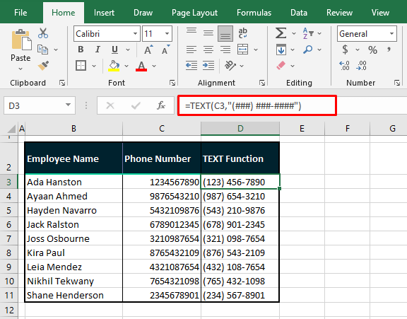
TEXT function with Different Digits Numbers

Have you thought about what you'd have to do if you had phone numbers from different countries with varying digits? How would you handle formatting 9 and 10-digit numbers? You could use the formula above but that would enclose the initial 2 digits of the 9-digit numbers instead of the 3-digit area code in parentheses. That’s where the IF function can come in handy.

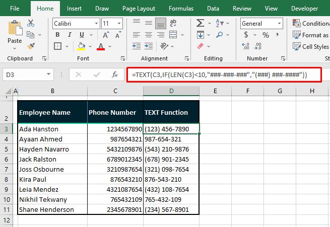
In our second example case, we have 10-digit and 9-digit phone numbers belonging to two different countries. We want the numbers from both countries to be distinguished by way of format. This can be done using the TEXT function with the IF function. Below is the formula using the TEXT function to convert phone numbers in two different formats along with the IF function:

Let’s describe the mechanics of this formula. The LEN function returns the number of characters in C3 i.e. 10, and passes the result to the IF function. IF checks whether the number is less than 10 or not. If true, the TEXT function formats the number with the first provided format i.e.:

If false, like in this instance, the TEXT function will use the second format to format the number i.e.:

Descriptively, the TEXT function is to format the value in C3 according to the provided format. The format will depend on the result of the IF function. If the number of characters in C3 (as counted by the LEN function) is less than 10, then the TEXT function will choose the first format. Otherwise, TEXT will choose the second format.

We will extend the formula for all the numbers to format them as phone numbers:

Numbers with Leading Zero

It is not unknown that many country calling codes start with 0 but do you know what will happen if we try entering such a phone number in Excel? Try it. The zero(s) won’t show up and this is not some Excel magic but an Excel nuisance. It’s alright, you’re not stuck. Let’s see a few ways below on how to work with phone numbers that start with 0.

Pre-formatted with Custom or Text Format

The cells in which the phone numbers are to be added can be preformatted with a Custom format to keep the leading zero in place. The formatting code needs to be in zeros. The number of zeros depends on the number of digits in the phone number. E.g. if we want 11-digit phone numbers we will enter this formatting code:

This will make sure that any entered value in the preformatted cells will be a total of 11 digits so that even if you enter 10 digits, automatically the first will become a zero.

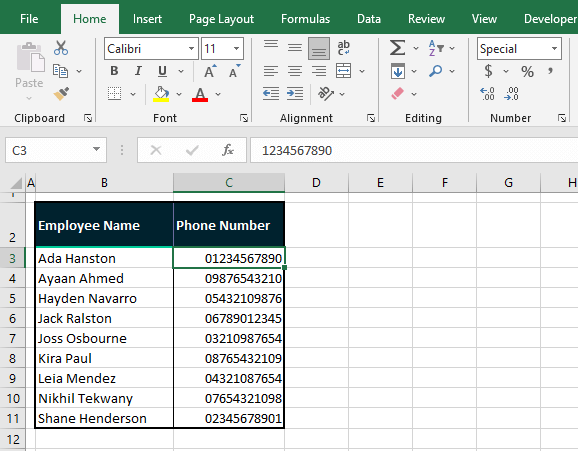
If the format is an incidental match for a Special format, it will show up in the Number Format bar.

This works either way, before or after entering the numbers. To add a leading zero to existing 10-digit numbers, apply the custom format using the formatting code above. Likewise, the target cells can be preformatted with a Text format to hold the leading zero in place but unlike custom formats, this will only work retrospectively.

Using Signs

Entering numbers with signs (e.g. hyphens, parentheses, spaces) will make Excel accept the numbers as text and would not, therefore remove the leading zeros. But sadly enough, a leading plus sign, like a zero, will not make it to the final value. This is because Excel treats a number with a leading plus sign as a positive number which does not require a plus sign to be displayed.

If you must use a leading plus sign, the way around that again is to use Custom format. To add a plus sign to 10-digit numbers, you can use the following format:

The results of using this format:

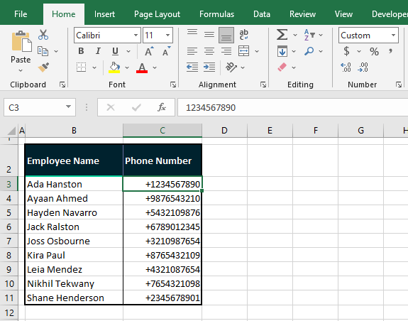
A leading plus sign can also be added with a preceding apostrophe. You'll get the idea by reading the next section.

Using Leading Apostrophe

One of the oldest tricks up the sleeve to force Excel to accept any entered value is to use a leading apostrophe. The leading zero will be retained along with the phone number when entered after the apostrophe and the apostrophe itself won’t show:

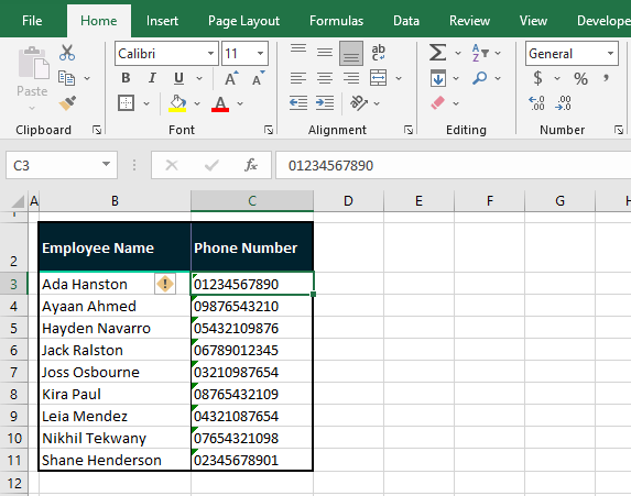
Note: The errors can be removed by selecting the cells, clicking on the error icon, and selecting the Ignore Error option.

Round-up now. As we see it, Excel has a few set ways if you are formatting phone numbers. If those don’t float your boat, you can always resort to other tricks and custom tweaks to arrive at your desired format. All you need is a go-getter attitude. How about we go get another clump of Excel tips and tricks? On it!