How to Highlight Weekends in Excel (In 3 Easy Ways)

Have a great weekend! If the title didn’t do it, that should drop a hint on what’s coming up today. Yes, we’re learning how to highlight weekends in Excel, and trust us when we say it looks nothing like this angry green buddy up here.

You will find it most convenient to highlight certain days of the week to spot a pattern, for analysis, timelines, schedules, etc. You may be trying to find out the weekend or weekday dates or working days and it’s far easier to have them pop out in color instead of having the weekday names written down.

Our interest today is the weekend and we will leave the job to Conditional Formatting to find and highlight the weekends for us. The hands helping Conditional Formatting search for the weekends are going to be the WEEKDAY, WORKDAY, and WORKDAY.INTL functions.

These three will cover the inclusion of user-provided holidays and selection of weekends in case your weekend differs from the general Saturday and Sunday. Let’s move on to what we’re working with and talk about the example we will use to carry out our Excel testing.

Example

Scratching the surface of the technical part of things, here is the example we will use as a basis to demonstrate how to highlight weekends in Excel:

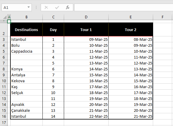
We are comparing two 2-week tour schedules. Tour 1 begins on the 9^th of March with the rest of the schedule in column D. In column E we have the schedule for tour 2 which commences on the 8^th of March. To compare which schedule gives us a wiser utilization of the weekend and rest days, it would be preferable to have the weekend days highlighted first.

The Long Date format displays the day of the week with the date but highlighting immediately categorizes the data. For comparison’s sake, we will be highlighting weekends to identify which tour schedule suits us best.

Pro tip: This guide shows how to use formulas through a dialog box. If you want to experiment with the formulas and their results, try using the formula on the active worksheet first. Then copy-paste the amended formula in the dialog box.

Let’s get highlighting!

Method #1 – Using WEEKDAY Function

Highlighting weekends is an easy game using the WEEKDAY function with Conditional Formatting. In the WEEKDAY function, you can set which day is the first day of the week for you. According to that, the WEEKDAY function will return a number from 1 to 7, representing the day of the week of the provided date.

Conditional Formatting can be used to change the appearance of a cell according to its value which distinguishes it from other cells, making it easier to spot trends and patterns. The feature of Conditional Formatting we’re interested in today is Highlight Cells. Using the WEEKDAY function in Conditional Formatting, we will highlight the cells with the weekend dates. Find more details on this with the steps below:

• Select the cells with the dates.
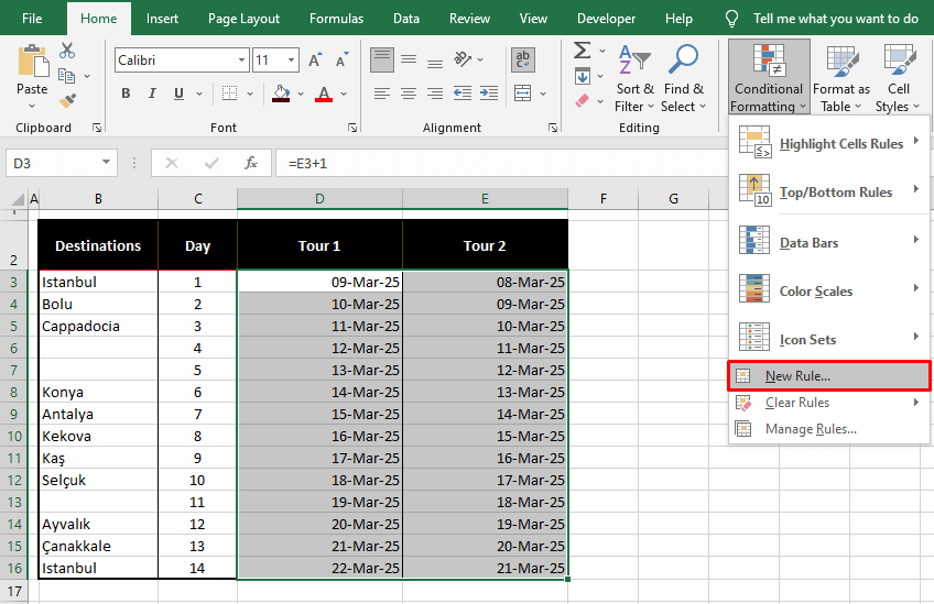
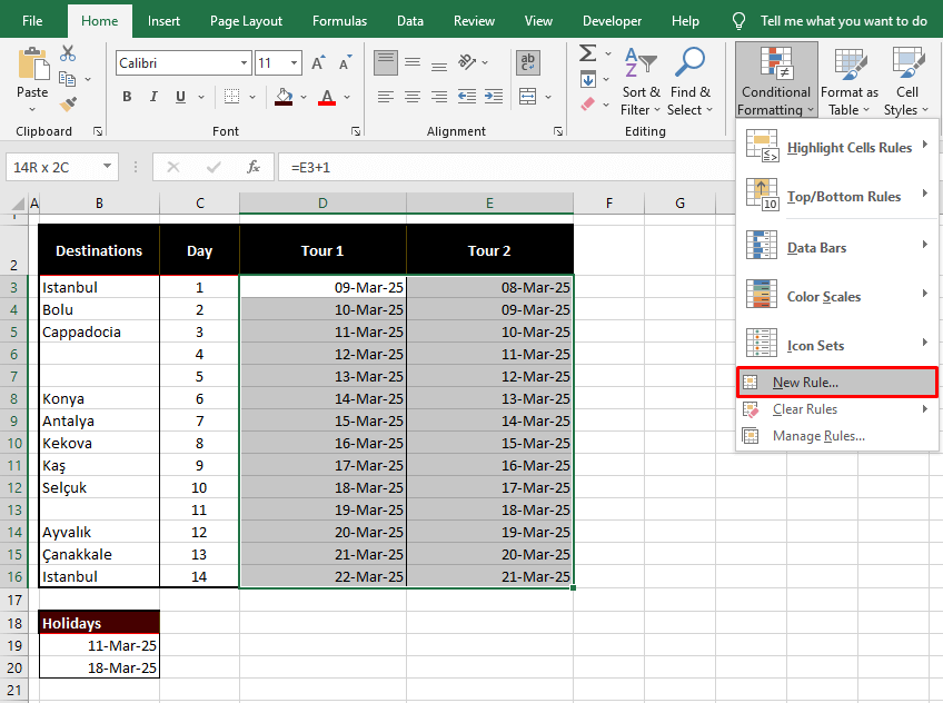
• In the Home tab, select the Conditional Formatting icon in the Styles
• Select the New Rules option from the menu.
• 
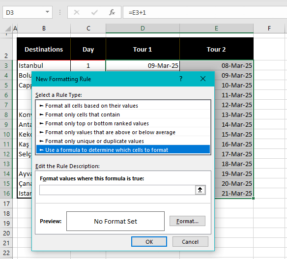
• This will open the New Formatting Rule dialog box.
• In the dialog box, click on the Rule Type – Use a formula to determine which cells to format.
• 
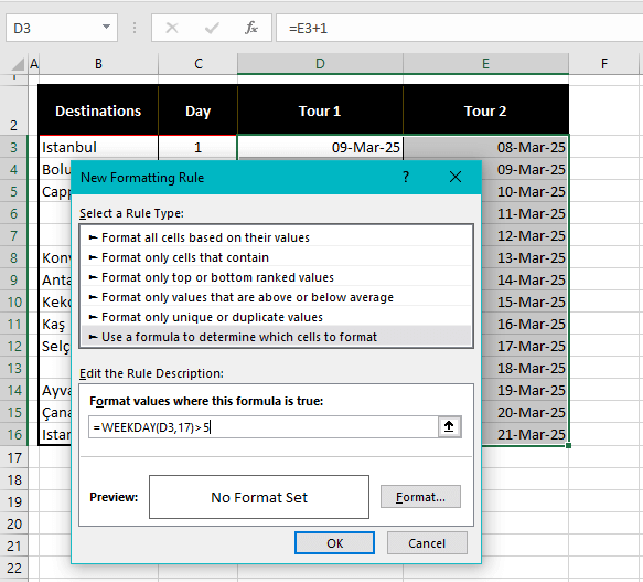
• In the provided text box, paste the following formula:
• =WEEKDAY(D3,17)>5
  
• Click on the Format button to open the Format Cells dialog box. Use the Fill tab to set the color fill for the highlighted cells.
• Click on the OK button of the Format Cells dialog box when done.
• 
• Select the OK button of the New Formatting Rule dialog box.

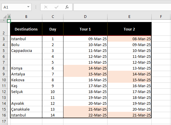
All the weekend day cells in the selection will be highlighted:

How the formula works

The WEEKDAY function starts with the date in D3. From the week options listed by WEEKDAY, we have selected 17 – this option takes Sunday as the first day of the week, making Friday and Saturday the weekend. With this option, Sunday will be represented by the number 1 and the weekend i.e. Friday and Saturday will be represented by 6 and 7 respectively.

Now how will this work? WEEKDAY will check the date in D3 – 9^th March. This falls on a Sunday so WEEKDAY will return the number 1. In the remaining part of the formula, WEEKDAY’s results will be tested to be greater than 5. If this is true, only then will the cell be highlighted. Since 1 is not greater than 5, Conditional Formatting does not highlight D3.

Notes:

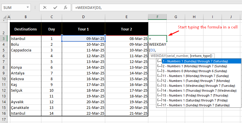
• To view the week options for the second parameter, start by typing the formula in a free cell. The Formula AutoComplete will display the week options:
• 
• On the other hand, if it's the weekdays you want to be highlighted, set the formula to highlight all the cells whose WEEKDAY result is less than 6. Use this formula:
• =WEEKDAY(D3,17)<6
• For highlighting a specific day, let’s suppose we want to highlight Friday, change the symbol to an equals sign. With our selected week option i.e. 17, Friday will be day number 6. Hence, we need WEEKDAY’s result to equal 6. We’ll use this formula:

Method #2 – Using WORKDAY Function

Highlighting weekends is doable using the WORKDAY function with Conditional Formatting and you also get the option of adding holidays to the mix. The WORKDAY function returns the serial number that represents the date before or after a given number of workdays.

WORKDAY can take a parameter for holidays that will be excluded when counting workdays up to a certain date. Making use of this option, we can use the WORKDAY function with Conditional Formatting to highlight weekends and holidays. See the steps for this below:

• Select the range containing the dates.
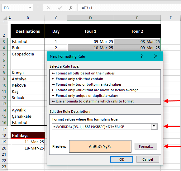
• Go to the Home tab > Styles group > Conditional Formatting icon > New Rule option to launch the New Formatting Rule dialog box.
• 
• Click on the last option in Select a Rule Type – Use a formula to determine which cells to format.
• Add this formula in the Format values where this formula is true field:
• =WORKDAY(D3-1,1,$B$19:$B$20)=D3=FALSE
• Also set a highlighting color for the weekend date cells by clicking on the Format
• 
• Click on the OK

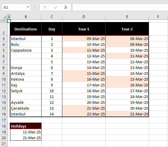
From the selected cells, all the weekend dates and holidays will be highlighted:

How the formula works

The expression "-1" in the first parameter returns the date before the date in D3. 1 day before D3 i.e. 9 March 2025 (which is a Sunday) is the 8^th of March 2025. Then, the number 1 in the second parameter will return the date of 1 working day after 8 March 2025. Since the 9^th is a Sunday, 10 March 2025 is the date we’re at now.

The holidays in B19:B20 (entered as an absolute reference in the formula with $ signs using the F4 key) do not overlap with the 10^th of March 2025 and so the result of the WORKDAY function is 10 March 2025.

Now the next part of the formula checks if the result of WORKDAY equals D3. In this instance, 10 March 2025 does not equal to D3, which means the result up until now is FALSE.

The final part of the formula checks whether the formula equals FALSE and if it does, D3 will be highlighted. Conditional Formatting highlights D3 as an off day.

Note: For highlighting weekdays, remove the “=FALSE” expression from the formula so that the cells will be highlighted as per the condition of the result of the WORKDAY function being equal to the date in the cell. The formula to be used in Conditional Formatting will be:

Using this formula, the weekday cells will be highlighted:

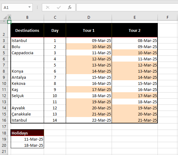
Did you notice anything different about highlighting weekends using the WEEKDAY and WORKDAY functions? Compare the results. The difference is that the WORKDAY function by default assumes Saturday and Sunday as the weekend whereas we had the option of choosing the weekend days with the WEEKDAY function. Want to include holidays and pick the weekend? Keep on reading.

Method #3 – Using WORKDAY.INTL Function

A very customized method of highlighting weekends involves the WORKDAY.INTL function The WORKDAY.INTL function works with custom weekend parameters and a given range of holidays to return the serial number of the date of an earlier or later working day.

You can consider this function a combination of the WEEKDAY and WORKDAY functions. Checks all the boxes, right? Let’s find out how to use it:

• Use the same steps as above for Conditional Formatting. In the New Formatting Rule dialog box, use the formula below:

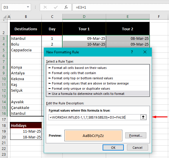
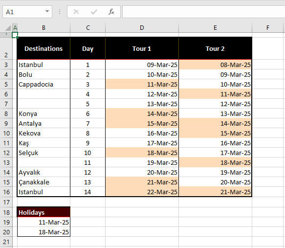
All selected cells whose WORKDAY.INTL result will be FALSE will be highlighted:

How the formula works

The formula works exactly like the one we used with the WORKDAY function, only that here you can see an additional parameter, the third one, the number 7. This is the weekend parameter for Friday and Saturday as the weekend days, selected from the weekend options in the Formula AutoComplete.

Let’s run through the formula. The date in D3 i.e. 9 March 25 (Sunday) is taken back one day deducting 1 from it, leading to 8 March 25. According to the weekend parameter set in the formula (i.e. 7) and excluding the holidays in B19:B20, the second parameter adds one working day to this date, leading to 9 March 25 (Sunday).

The formula then checks if the 9 March 25 equals D3 which it does and results in TRUE. This does not meet the criterion for highlighting as only the cells with the formula resulting in FALSE will be highlighted. D3 remains unhighlighted.

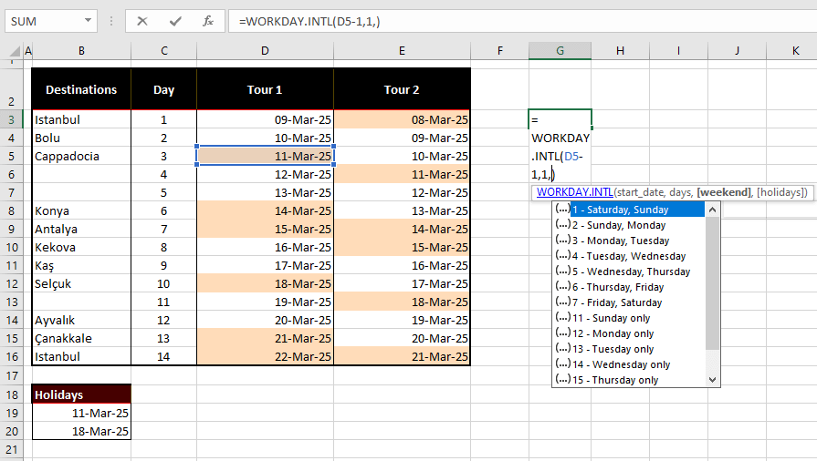
Note: Type the formula in an empty cell to view the weekend parameters in the Formula AutoComplete:

However the weekend, this is the tutorial end. Those were 3 ways on how to highlight weekends in Excel with some tricks on how to make the whole deal easier. Next time you’re trying to make ends meet by having the weekends on the sheet make themselves known, have a go at one of these formulas, adjusting them to your requirements. While you’re tweaking weekends, we’ll go tweak something else Excel.