How to Make Negative Numbers Show Up in Red in Excel

We have 3 quick and easy ways for you today to have the negative numbers in your spreadsheets displayed in red. We’re using Conditional Formatting and a couple of options via the Format Cells dialog.

With a long display of numbers, it can quickly become confusing for your eyes to single out the negative numbers. The negative numbers could be representing expenses, debit or credit entries, or a negative difference between two amounts, and let's just say how significant that one little minus sign can be, financially speaking. Yes, these numbers are very important and that may be why you want them to show up a little more clearly than just with a hyphen as their prefix or parentheses as their enclosure.

This is what we have in today’s tutorial; highlighting negative numbers in red, leaving the positive figures as they are in the custom black. Now we’d like to crack into the methods of making negative numbers red in Excel.

Let’s get… reddening?

Method #1 – Using Conditional Formatting

With Conditional Formatting, the format of cells can be changed based on the specified conditions, according to the value of the cells. We will make use of this feature to highlight negative numbers in red by setting the condition to highlight numbers less than zero in red text. The steps for using Conditional Formatting to highlight negative numbers in red are below:

• First, you need to select the cells with the numbers, both negative and positive.
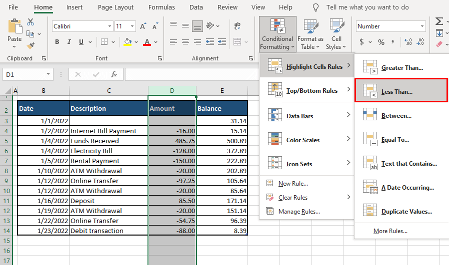
• In the Home tab, click on the Conditional Formatting button in the Styles. Select Highlight Cells Rules > Less Than… from the menu.

• A window will pop up where you need to specify the formatting condition. Type “0” in the first field and select Red Text from the following list. You can also select a different format such as Light Red Fill with Dark Red Text. This option will also highlight the cell in light red color fill.

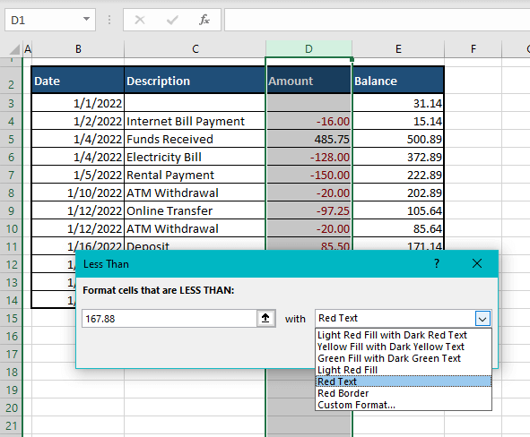
• Click the OK button when done.

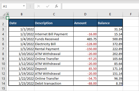
Now all the numbers less than “0” in the selected cells will be highlighted in red text:

Method #2 – Using Excel Number Formats

Excel has an assortment of formats for numeric values. Using the options in the Format Cells dialog box, we will display the negative numbers in red. Below are the steps for displaying negative numbers in red using the inbuilt Excel Number formatting:

• Select the cells with the numbers.
• In the Home tab, select the dialog launcher in the Number group (or press Ctrl + 1) to launch the Format Cells dialog box.

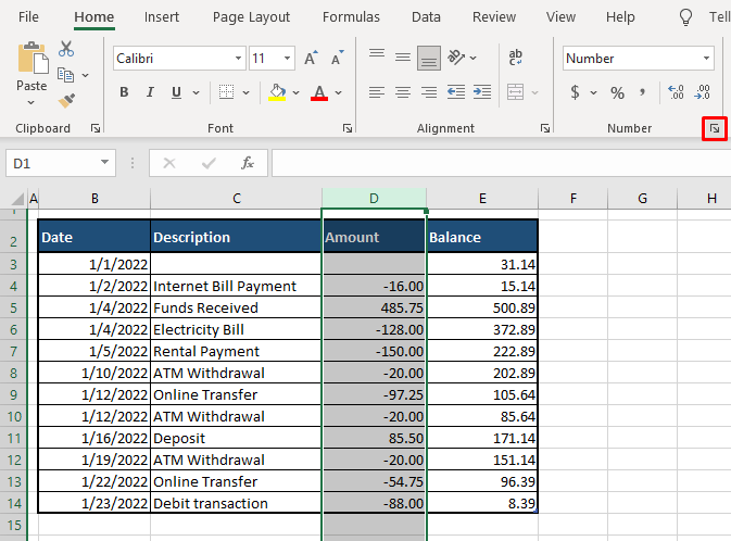
• Go to the Number category in the left panel and select the last option for negative numbers.

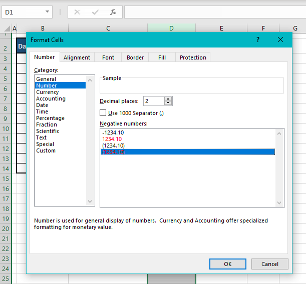
• Click on OK.

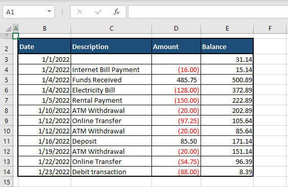
This option will display negative numbers in red and enclosed in parentheses. If you want a minus sign (hyphen) instead of the parentheses, you can head to the Custom category. For details on what to do in the Custom category, read below.

Method #3 – Using Custom Number Formats

This method is similar to the one above which uses the Number formats in the Format Cells dialog. But this time, we’re heading to another category to customize the results. The complete steps for using custom number formats to make negative numbers red are as follows:

• Select the range where you want the format to apply.
• To open the Format Cells dialog box, select the dialog launcher in the Home tab’s Number group or press Ctrl + 1.

• Now you can go to the Custom category and directly copy-paste this code:

OR

But to give you a better idea of the way this works, let’s select a preset option and customize that.

• In the Number tab, select the Number. Click on the second option with the number in red text and then select the Custom category from the left panel.

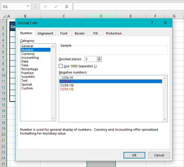
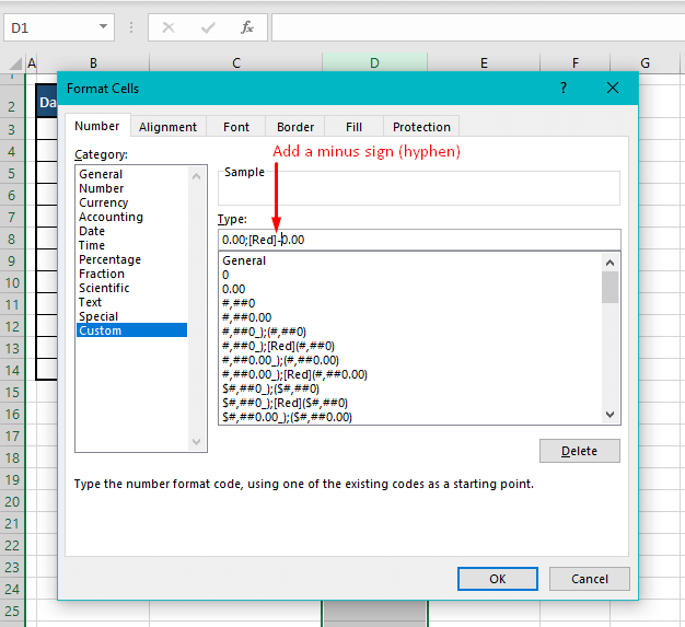
• In the Custom category, you will see the code for the number format of your selection in the Type: field. All you need to do is add a hyphen to this code.

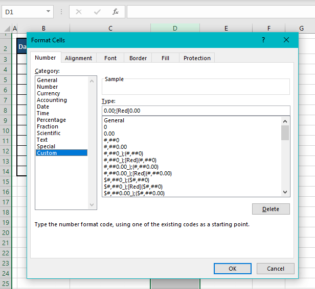
• Add a hyphen sign to the code in the Type: field between “0.00;[Red]” and “0.00”.

• Click on OK.

The negative numbers will be displayed in red with a minus sign.

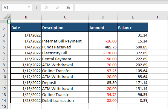
Wasn’t that easy? So easy that now we’re done! That was our quick guide today on how to make negative numbers show up red in Excel (no Excel blood was shed in the making of this tutorial). Next time you want your expenses to jump out at you in red alert or simply when you want a clear divide between negatives and positives, give one of the methods above a go. Before this sounds any more medical, we’ll show up with more positive solutions for your Excel hitches in no time!