The Formula Bar in Excel has more to it than what meets the eye and today's tutorial will give you a rundown on it. (A run down and up if we're honest!)
The Formula Bar is one of the core features of Excel and we will guide you on what it is, how to hide/display, expand/contract it, and how to use formula bar icons.
Let's get formulating!
What is the Formula Bar in Excel
The Formula Bar in Excel shows the formula or value of a selected cell and can be used to edit any selected cell's value. In the case of a formula, the cell will display the result while the Formula Bar will show the formula. The Formula Bar will display the underlying value of a cell while the cell may show a formatted value.
As soon as you start typing in a cell, the Formula Bar will start displaying the contents. The Formula Bar shows the contents of a single cell and therefore, in a selected range, the Formula Bar will show the contents of the first selected cell.
It is located between the column headers and the Ribbon, to the right of the Name Box. The given size of the Formula Bar is not a limitation, and it can be expanded or contracted vertically as well as horizontally. It is possible to completely hide and restore the Formula Bar.

How to Hide Formula Bar
By default, the Formula Bar is displayed in Excel. You might want to temporarily hide it to fit a few more rows into the worksheet space. Also, when you start typing in a cell, you are using the cell to add the contents instead of the Formula Bar so you might find that you prefer to hide the Formula Bar while working, making more rows visible too.
The Formula Bar can be hidden using the option in the View tab (by the mouse or keyboard) or in Excel Options. The methods are given below.
Method #1 – Using Ribbon Menu
Hide the Formula Bar in Excel by changing the view of the spreadsheet using the View tab in the Ribbon menu. The process is complete in a couple of clicks, here's what to do:
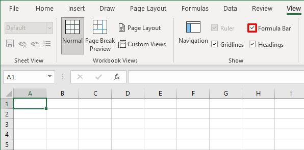
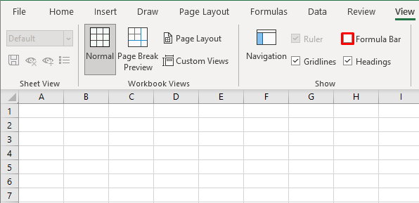
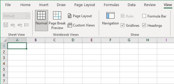
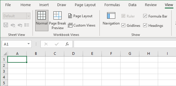
- Go to the View tab in the Ribbon and click on the Formula Bar checkbox in the Show
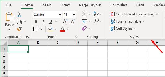
- With the Formula Bar box unchecked, the Formula Bar has been removed from view:
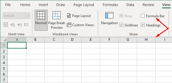
After the Ribbon, the column headers have shifted upward, taking place of the Formula Bar. Check the Formula Bar box any time in the View tab to bring the Formula Bar back.
Method #2 – Using Excel Options
The next method of hiding the Formula Bar in Excel is through Excel Options. Find out how to access Options in Excel and how to use it to remove the Formula Bar from display with the steps given ahead:
- Select the File tab from the set of tabs above the Ribbon.
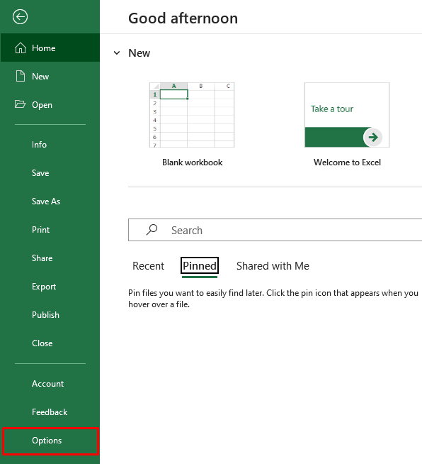
- Click on Options from the bottom of the left side pane.
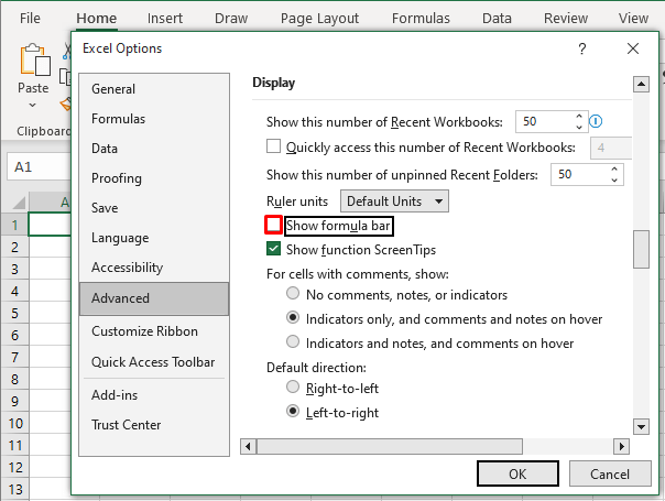
- From the left panel, select the Advanced
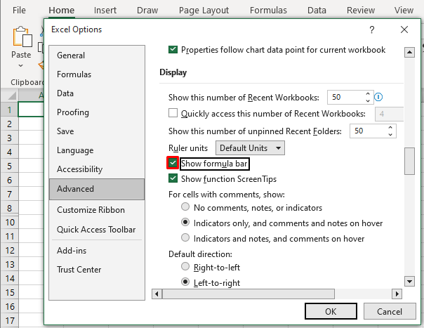
- Scroll down to the Display section and unmark the Show formula bar
- Click on the OK button to apply the setting.
This will close the Excel Options dialog box, return you to the worksheet and hide the Formula Bar from display.
Method #3 – Using Keyboard Shortcut
Use the keyboard instead of the mouse to quickly remove the Formula Bar from view. This keyboard shortcut takes the route of the View tab to hide the Formula Bar. The keyboard shortcut for hiding the Formula Bar in Excel is:
Alt, W, V, F
Enter the keys above one after the other.
Alt key displays the shortcut keys for the tabs.
W key selects the View tab.
V, F keys select the Formula Bar checkbox.
The keyboard shortcut has led to the previously checked box being unchecked and therefore hiding the Formula Bar:
How to Show Formula Bar
If the Formula Bar has been hidden, using any one of the methods above will bring it back. While cells are mostly edited by direct typing, with the values of the surrounding cells, the contents of the active cell may become confusing, making the Formula Bar a better choice for editing data.
To restore the Formula Bar above the worksheet area, use one of the methods listed below.
Method #1 – Using Ribbon Menu
The Formula Bar option in the View tab is used to hide and unhide the Formula Bar in Excel. To unhide the Formula Bar:
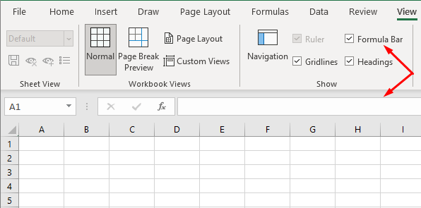
- In the View tab's Show group, check the Formula Bar box which should be unchecked at this point:
- After check-marking the box, the Formula Bar will be added back below the Ribbon:
Method #2 – Using Excel Options
To show the Formula Bar in the spreadsheet, you can use Excel Options. Follow these steps to bring the Formula Bar back on display:
- Select the File tab and then Options from the left.
- Next, select the Advanced tab and tick-mark the Show formula bar
- Hit the OK button to confirm the setting and close the dialog box.
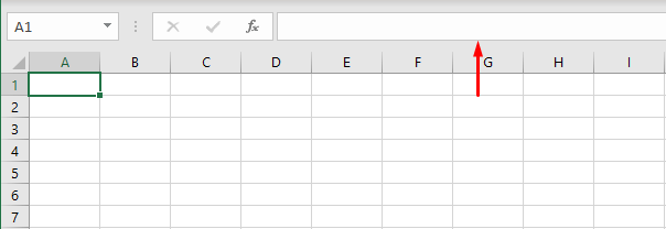
The Formula Bar will return above the column headers:
Method #3 – Using Keyboard Shortcut
Use a keyboard shortcut to display the Formula Bar in Excel. This keyboard shortcut will lead to the View tab to select the Formula Bar checkbox. Enter the keys below in succession:
Alt, W, V, F
The Formula Bar box will be checked, showing the Formula Bar in the spreadsheet again:
How to Expand or Contract Formula Bar
The Formula Bar is not small by any means and can house a fairly long formula or cell value. But for longer formulas or cell values with line breaks, you will find that expanding the Formula Bar is much easier to work with. Also, when you're working with multiple windows and have downsized your Excel window, the Formula Bar will consequently have lesser space than before.
The first suggestion to resize the Formula Bar is to resize your spreadsheet window. The drawback of that however is that a smaller window will not contract the Formula Bar to display the complete value of the cell or the formula; if either is too long, it will be hindered from view. Therefore, if it's preferable not to resize the window, the Formula Bar can be contracted and expanded vertically in a couple of ways as well as horizontally. All three ways cater to resizing the Formula Bar differently. Details are given below.
Using Expand/Collapse Arrow
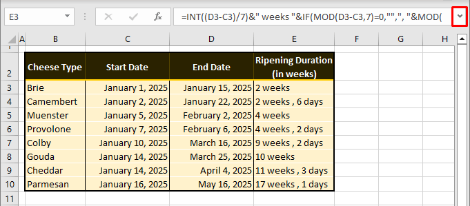
The small arrow at the end of the Formula Bar is for expanding or collapsing the Formula Bar. In the example ahead, the formula in cell E3 cannot be viewed completely. We will expand the Formula Bar to view the formula using the arrow:
The Formula Bar has expanded by another line and displays the whole formula now:
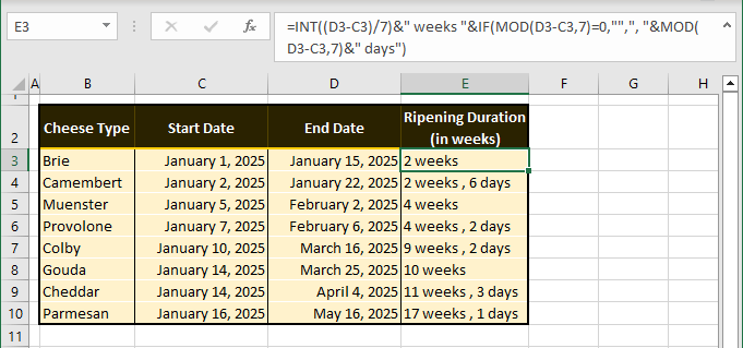
Note: This arrow will expand the Formula Bar to the size last set by the resizing arrow (coming up in the section ahead). If you haven't used the resizing arrow before, the expanding arrow will only extend the Formula Bar by one more line.
Use the same arrow to contract the Formula Bar back to a single line:
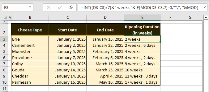
Pro tip: Use the keyboard shortcut Ctrl + Shift + U to expand/collapse the Formula Bar. The shortcut toggles the Formula Bar's expand/collapse arrow.
Using Resizing Arrow
If the expand/collapse arrow isn't giving you the right amount of view in the Formula Bar, you can expand the bar to the desired setting using the resizing arrow. You may be familiar with resizing arrows used on windows or objects. Two such arrows are available for the Formula Bar and they work to resize it vertically and horizontally (the latter explained in the next section).
This can be used as a preset for the expand/collapse arrow. We'll let you know how. For now, have a look at the example case below. We have an address given in B13. The Formula Bar makes it evident that the address in B3 contains at least one line break as we cannot see the complete contents.
If we use the expand/collapse arrow at this point, we will only be able to view one more line and ideally, we should be able to view four in this case. To expand the Formula Bar to our preference, we will resize it instead by placing the cursor at the lower edge of the bar until a double-headed arrow appears:
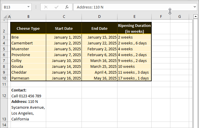
Click and drag the Formula Bar using this arrow and extend it to the preferred length (four lines as per our example case). Now the Formula Bar will display the full contents of B13:
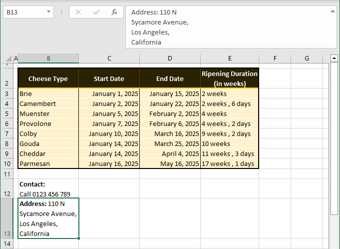
Use the same double-headed arrow to contract the Formula Bar to the preferred point or click the expand/collapse arrow once to restore the single-line Formula Bar.
After this, when you use the expand arrow, the Formula Bar will be extended to four lines instead of two since the expand arrow extends the Formula Bar to the last size set by the resizing arrow.
Resizing Horizontally
The Formula Bar in Excel can also be resized horizontally. You may need to expand the Formula Bar if you contracted it previously. Contracting it horizontally gives more room to the Name Box to display a longer name (e.g. of a range or cell).
Below in the example, we have named all the cells containing contact numbers as PhoneNumber, PhoneNumber2, and onwards so that they are easier to find. The Name Box with its current size can't display the full name so we will resize the Formula Bar.
To contract the Formula Bar horizontally, place the cursor on the 3-dot menu icon between the Name Box and the formula bar icons until a double-headed arrow shows:
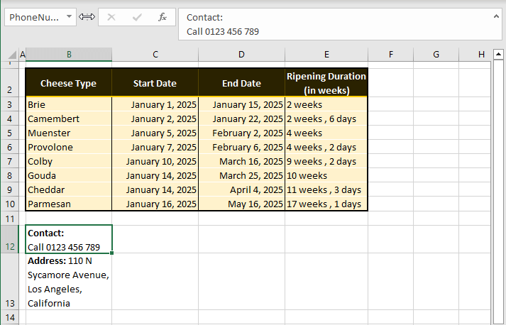
Click and drag to adjust the size of the Formula Bar. You can see below that the Formula Bar has contracted, expanding the Name Box:
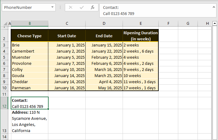
Use the resizing arrow to expand the Formula Bar again or double-click the 3-dot menu to restore it to the default size.
Formula Bar Icons
The formula bar icons are used for actions regarding the Formula Bar. The icons are situated before the Formula Bar itself, on the right of the Name Box:
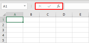
Now would be a good time to tell you what these icons represent and how they can be used. As a rule, the icons are usable if they change color from gray when you hover the cursor over them. If the icon remains gray, it is unusable at that time.
Cancel button – The Cancel button works as a replacement for the Esc key. It is only activated in cell edit mode i.e. the active cell (whether via the Formula Bar or the cell). Clicking on the button exits cell edit mode while the cell remains selected. If any changes have been made to the active cell, the Cancel button will revert the cell value to the value before editing, maintaining the cell selection. That means that the button only works for the edits of the active session.
Enter button – The Enter button works a bit like the Enter key but only for the active cell and also maintains the cell selection. If the button is used without making any changes to the active cell, cell edit mode will be exited while the cell remains selected. If the button is used after making changes to the active cell, the cell will take on the edited value, cell edit mode will be exited and the same cell will remain selected.
Insert Function button – The Insert Function button is used for inserting a function in a cell. It's kind of like a functions encyclopedia. The button (or the Shift + F3 keys) opens the Insert Function dialog box where you can search for a function.
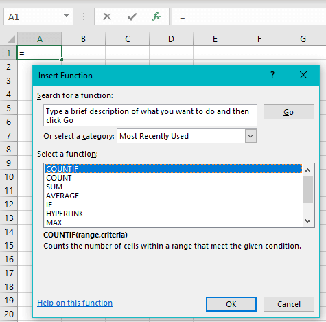
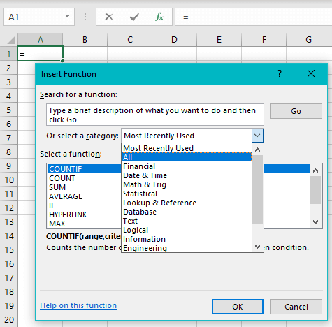
Search for a function by category. The default display of the functions is the Most Recently Used category. Other categories are groups of functions and can help you find a function according to those groups. The All category will alphabetically list all the functions.
Another easy way is to search for a function by entering a description. Functions with matching descriptions will be displayed for you to choose from. E.g., for counting blank cells, we can type the description "count blank cells" and hit Go. These would be the results:
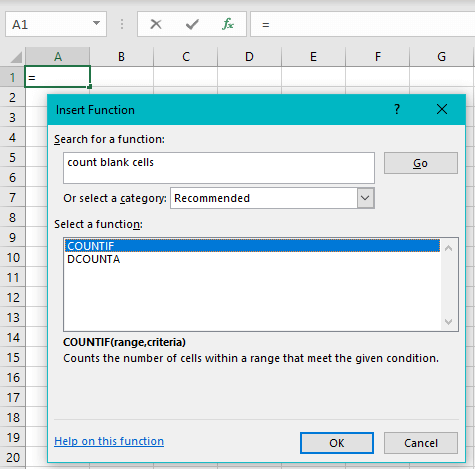
The syntax and description of the selected function will be shown in the dialog box. (For more help, click on the Help on this function link at the bottom of the dialog box and it will lead to the Microsoft website.) Select a function by double-clicking it and you will be led to the Function Arguments dialog box which will aid you in forming the formula correctly with the arguments and will also break down the results:
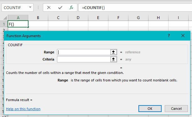
When done, the OK button will enter the formula and display the results in the selected cell on the worksheet.
The Insert Function button does not need an active cell to be usable. In the active cell, it can only be used if the cell is either blank or contains a formula. With any other value present in the cell, the Insert Function button will remain disabled.
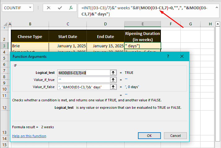
The button can be used on any selected cell (without entering cell edit mode). If the button is used on a cell containing a formula, the Function Arguments dialog box will open with the function that the blinking cursor is positioned on. Using this case as an example, if we keep the blinking cursor at the IF function in the formula, and select the Insert Function button,
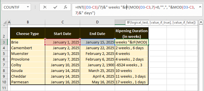
The IF function will be emboldened in the Formula Bar while the Function Arguments dialog box opens with the details of the IF function in this particular formula:
Note that while Insert Function can overwrite a cell's value, it cannot overwrite the format; the function used will result in the set cell format (if any).
Today we got up close and personal with the Formula Bar in Excel. Who should our next guest of honor be? We'll get busy with that while you can experiment with the new bits and bobs you learned about the Formula Bar. Enough tricks we got there to keep you occupied? Only one way to find out. Ready? Tricky? Go!
