Excel TEXTJOIN Function – How To Use

The TEXTJOIN function joins text or strings from multiple cells into one cell separating them using the given delimiter with an option to include or ignore empty strings. It was first introduced in Excel 2016.

The TEXTJOIN function combines the values while adding the specified delimiter between each text. The return value of the TEXTJOIN function is always in text format.

Syntax

The syntax of the TEXTJOIN function is as follows:

Arguments:

The TEXTJOIN function accepts three mandatory arguments. The details of each are mentioned below:

'delimiter'- This is a required argument. The delimiter is a text that we wish to add between each text to be combined. The input value of the delimiter can be passed directly in double quotes or as a cell reference. If the value of the delimiter argument is a number, the TEXTJOIN function treats it as a text value.

'ignore_empty' – This is a boolean argument that accepts TRUE or FALSE as its input value. It is a mandatory argument and cannot be left blank. We can also use 1 or 0 as input values which indicate TRUE or FALSE, respectively. TRUE indicates that the function shall ignore any blank cells and does not include them while joining text strings, whereas FALSE indicates that empty strings must be included in the combined string.

'text1' – This argument is also mandatory and accepts the first text value that is to be combined. It can be a cell reference or direct value in double quotes.

'text2, text3, text4….' – These are subsequent text values that are to be joined together with text1. These are optional arguments depending on the number of text values to be combined.

Important Characteristics of the TEXTJOIN Function

Some of the essential features of the TEXTJOIN function are given below:

• If the value of the text argument contains number formatting, the return value of the TEXTJOIN function removes the formatting and returns the joined string with the original data.
• If the return value of the TEXTJOIN function exceeds 32767 characters which is the cell limit in Excel, the function throws a #VALUE! error.
• The maximum number of optional text arguments that are accepted by the TEXTJOIN function is 252.

Examples of TEXTJOIN Function

With a few mandatory arguments making up the TEXTJOIN function, let's understand the functionality of each one of them using some examples. Here, we have taken simple sample data with varying input values for each argument.

In the first example, we are simply concatenating two values in cell B3 and C3 separating them with the delimiter "!" mentioned in cell D3. The value of ignore_empty is FALSE, which means we will include the empty cells. The return value is simply all three values combined.

In the second example, we are combining a range of values from B3 to C7. This example also indicates that the TEXTJOIN function can also be used with array values. As seen in the return value, all the values from B3 to C7 are joined with the mentioned delimiter. As the ignore_empty is TRUE, the function ignored the empty cell (B6).

The third example is a classic case of the TEXTJOIN function converting a column to a string. Similarly, the fourth example is also combining all the numbers in column C. The TEXTJOIN function works with numbers but treats them as text values.

In the last example, we are combining the value in two cells but without a delimiter. As the delimiter argument is mandatory, we pass an empty string instead. The result is a simple concatenation of two values.

Now that the basic functionality of the TEXTJOIN function is clear let's move on to some useful applications of the function.

Example 1 – Combining Address Using TEXTJOIN Function

In this instance, we have all our employees' personal data, including full name, street name, city, state, and zip code. As the holiday season is approaching, we wish to mail all the employees their gift hampers. For the complete mailing address, we can simply combine data from all the cells using the TEXTJOIN function.

We will compile the complete address with commas (,), combining cell B3 to F3 while ignoring the empty cells. The formula will be as follows:

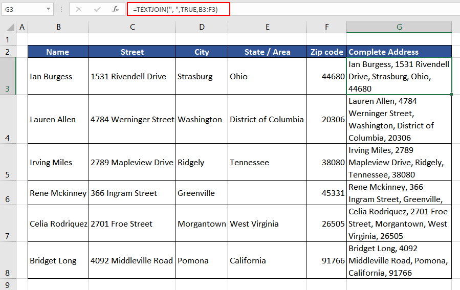
In the above example, we have understood how to use the TEXTJOIN function to join cells with the same delimiter. Further, we will explore the use of the TEXTJOIN function if more than one delimiter is to be used to join data.

Example 2 – Creating Email ID Using TEXTJOIN Function

In this instance, we have the list of new joiners, and the global HR team has the task of creating email IDs for everyone as per their country's domain name. The data includes first name, last name, and the country's domain name. As per the company's convention, the syntax of the email ID is 'firstname.lastname@domainname'.

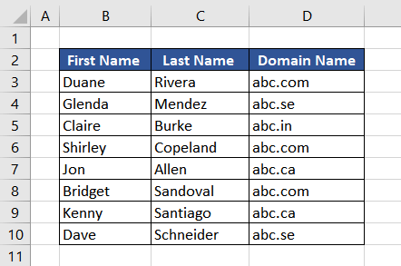
Using the TEXTJOIN function, we can join the first and last name using a dot (.) and combine the last name with the domain name using the at sign (@). As the names are in the proper case, we will also add the LOWER function while using the text argument so that the final email ID is in lowercase. The two delimiters (dot and at sign) will be used as array constants in curly brackets, each delimiter enclosed in double quotes, separated by a comma.

The formula used will be as follows:

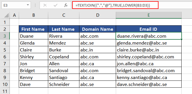
Example 3 – TEXTJOIN Function with Dates

In this scenario, we have the names and dates of birth of people. We now wish to join both using a line break. Looks like an easy task using the TEXTJOIN function. Let's see how the function behaves when joining text with dates.

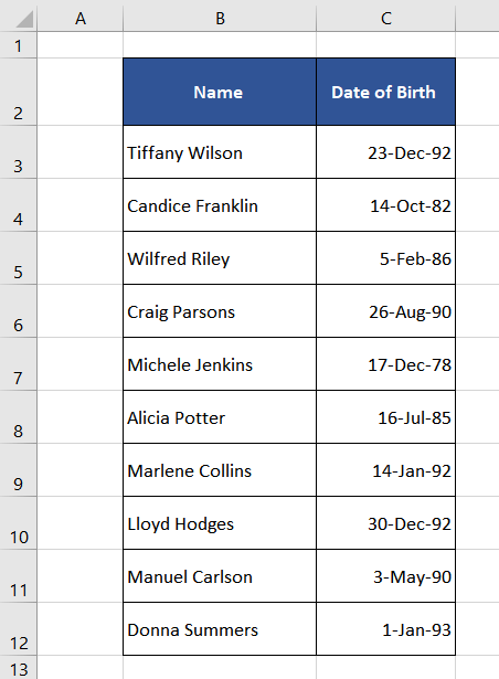
The formula used will be simple where the value of the delimiter will be a line break which can be inserted using the CHAR function. 10 is the character code that corresponds to a line break when using the CHAR function. We will include CHAR(10) in the formula to enter a line break and the complete formula is:

The delimiter is set as a line break with CHAR(10). Empty cells will be ignored with the usage of TRUE in the second argument. With those parameters, the names in column B and the dates in column C will be joined with the TEXTJOIN function.

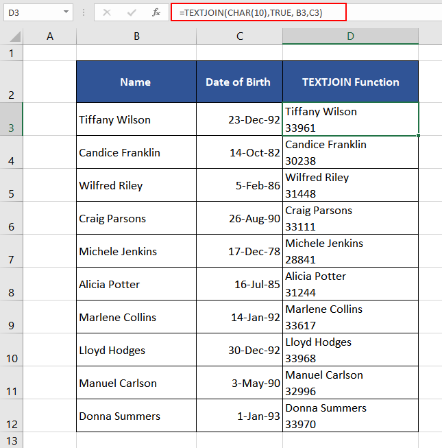
As we can see in the return value, all the date formatting is lost. This is because the return value of the TEXTJOIN function is always in text format and dates as we see in Excel are mere formatting and in actuality, it is stored as sequential numbers.

To ensure that the date formatting stays, we can make use of the TEXT function with the format "dd-mmm-yy". The formula used will be as follows:

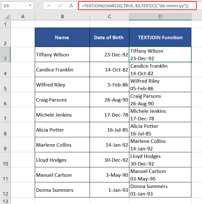
Now, the combination of name and date of birth looks presentable, and the date formatting remains intact.

Example 4 – Conditional TEXTJOIN Function

As the TEXTJOIN function operates well with arrays, we can also use it to combine the contents of two or more cells conditionally. Using the IF function, we can evaluate the condition and accordingly return an array of values to the text1 argument. Let's understand it better with an example.

Here we have the list of employees and the department they work in. The company is planning a team event, and we wish to segregate the team members as per their departments.

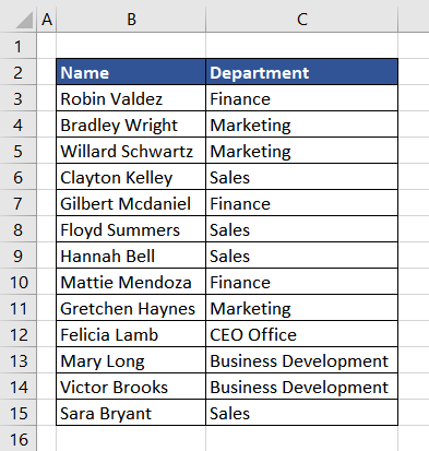
We will use the IF function to filter out the names in column B which match the given department name in column C. We will then use the return array as the input value for the text argument in the TEXTJOIN function.

To make things more refined, we have all the department names listed in column E (E3:E7).

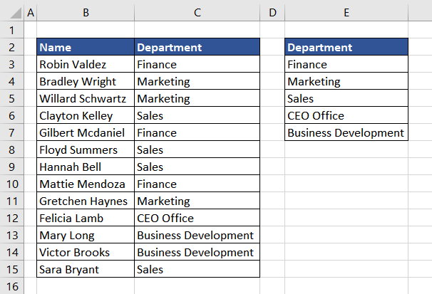
Our logic will be – If the value in column C matches the required department name, then return the corresponding value in column B, else do nothing.

The formula used will be as follows:

As we wish to compare each cell, we will add a dollar sign to each cell reference making it an absolute reference. Let's observe the return value of the IF function for better understanding.

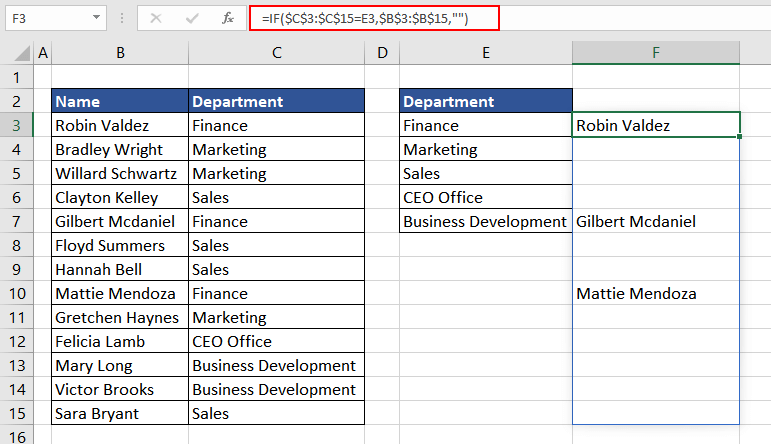
So far, the formula is listing the names corresponding to the department in E3, leaving the others blank. We can now use the TEXTJOIN function, combining all the return values with a comma (,) while ignoring the spaces, using the IF formula as the text1 argument. So that while the IF formula gets the names for the department, the TEXTJOIN function puts the list together with commas, ignoring empty cells.

The formula used will be as follows:

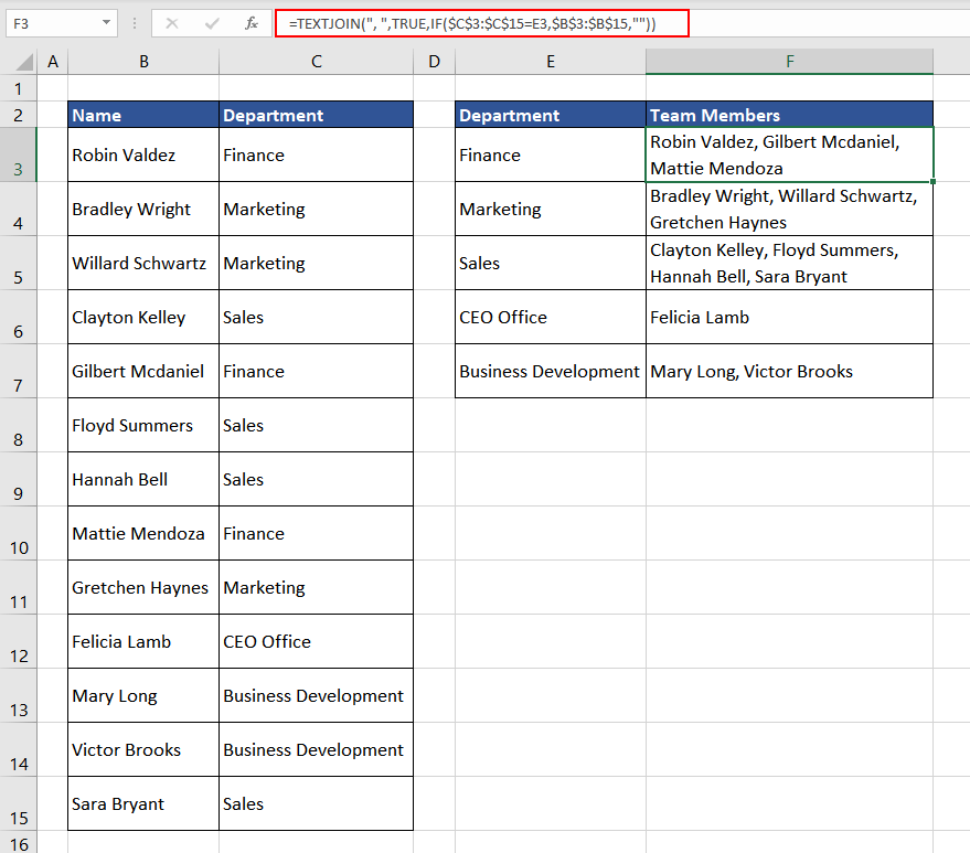
Now we have a better picture of each department's team members.

Example 5 – Reversing a String Using TEXTJOIN Function

Apart from the useful applications, the TEXTJOIN function can also be used to reverse a string. Combined with the MID function, we can easily reverse a string. The logic is to use the MID function to extract each character from the given string in reverse order and then combine them using the TEXTJOIN function.

To understand the concept, we will try to reverse the word "EXCEL" to "LECXE".

First, we will extract each character from the string in reverse order using the MID function. The formula used will be as follows:

This function will extract one character from the 10th position, then the 9th position, and then so on till the 1st position. We are taking 10 as an example to understand the concept.

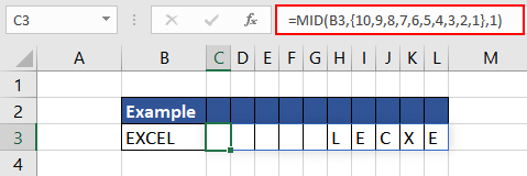
Now that we have all the characters extracted in reverse order, we will use the TEXTJOIN function without a delimiter while ignoring the empty cells. The formula used will be as follows:

As seen in cell C3, we have the reverse of the input string. But the problem with this formula will be seen if the length of the string exceeds 10 characters. To ensure that it can be used on any string, we can use the SEQUENCE function to create a sequence of numbers as per the length of the input string.

That sequence can be the input value for the starting position in the MID function. The Excel formula to create that sequence would be as follows:

The LEN function calculates the length of the input string, which is the number of rows required and also the starting value to create a sequence. The increment between each number would be -1.

Now let's use the above-stated logic and compile the final formula, which is as mentioned below.

Now we can easily reverse a string of any length.

TEXTJOIN Function vs CONCAT Function

Like the TEXTJOIN function, the CONCAT function joins text or strings into one cell. One major difference between the two is that in the CONCAT function, we must manually add each value along with the character we wish to insert between the values as a delimiter. On the other hand, while using the TEXTJOIN function, we can specify the delimiter just once and add the complete range of values in the formula.

Let's understand the difference between the TEXTJOIN and CONCAT functions using an example.

Here, we are trying to combine the values from cell B3 to B9 using a comma as a delimiter. Using the TEXTJOIN function as explained above, the formula used will be as follows:

On the other hand, in the CONCAT function, we had to manually add each cell and then mention a comma after each cell reference which is not the most efficient way when dealing with many values. The formula used will be as follows:

Hopefully, now all the aspects and applications of the TEXTJOIN function are clear. Practice the formula to discover new ways to use it while we work on another Excel function for you to learn.