Excel SORT Function – How To Use

The SORT function enables us to easily organize and rearrange the dataset as per our requirements. Using the function, we can quickly reorder the data in ascending or descending order based on one or multiple columns or rows.

The SORT function is an essential function when dealing with larger datasets as it simplifies the data by sorting it with defined parameters. New to the stage, the SORT function cannot be found in versions earlier than Excel 2021.

Syntax

The syntax of the SORT function contains four arguments that ensure that we can rearrange the given dataset as per the specified criteria. The syntax is as follows.

Arguments:

Details of the arguments and their roles are mentioned below.

'array' – This is a mandatory argument that accepts the value of the cell range or array that we wish to sort. The value of the array argument can be a static array, cell reference, or the return value of a function.

'sort_index' – This is an optional argument that indicates the column number or row number that must be used as a basis for sorting the data. If left empty, the default value of the argument is 1 which means the SORT function will sort by the first column or row depending on the input value of the by_col

'sort_order' – This is another optional argument that determines the order in which the data should be sorted. When left empty, the value defaults to 1 which rearranges the data in ascending order. When the value is set to -1, the data is sorted in descending order.

'by_col' – This is the last optional argument that accepts Boolean input values. This argument decides whether we want to sort by columns or by rows. By default, by_col is set to FALSE, which means sorting by rows. To rearrange the input data horizontally by columns, the value of the by_col argument should be set to TRUE.

Important Characteristics of the SORT Function

The most prominent characteristic of the SORT function is that it is dynamic in nature, which means when the data is altered in the input array, the same is reflected in the return data.

Some other noteworthy features of the SORT function are as follows.

• When you use the SORT function, it maintains the relationship between data in different columns or rows, ensuring that data stays correctly aligned even after reordering.
• If the value of the sort_index argument is out of range, the SORT function returns a #VALUE error.
• The sort_order argument only accepts 1 or -1 as the input value. If we enter any other value, the function throws a #VALUE error.
• Only omission or FALSE setting of the by_col argument results in the function sorting by row.

Let's go through some practical examples of the SORT function to learn how it helps us organize and rearrange data.

Examples of SORT Function

We know that the utility of the SORT function is to rearrange data based on columns. Let's delve into a practical example using a sample dataset to further grasp its functionality. Here we have a simple dataset containing names and corresponding scores.

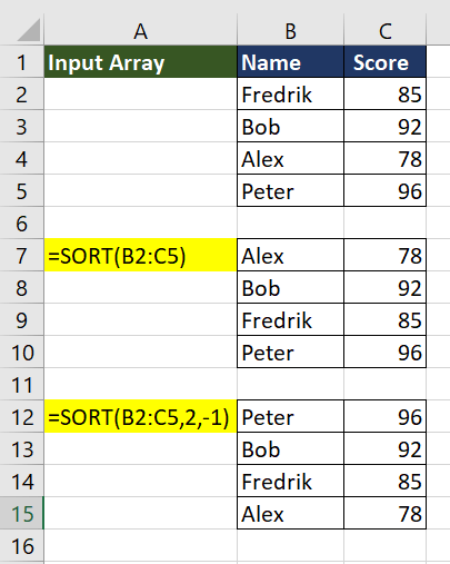
The first instance is a default view of the SORT function where we wish to rearrange the array B2:C5. As the other parameters are left empty, each argument assumes its default value and reorders the data as per the first column in ascending order, sorting by row. We finally have the dataset arranged in alphabetical order of the names.

The next example shows the context of other arguments. The formula takes the data in the cell range B2:C5, sorts it based on the values in the second column (column C) in descending order, and returns the sorted dataset. We finally have the data indicating top scorers to lowest.

With a foundational understanding of the function in place, let's progress to explore different methods and applications to make the most of it.

Example 1 – Simple Use of SORT Function

Imagine you are a teacher and it's the end of term. You now have all the students' grades in a dataset that includes their ID, names, and marks scored in three subjects. You now wish to do basic analysis such as finding out the top-performing student or the lowest marks secured in a subject.

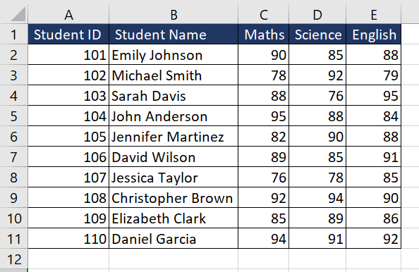
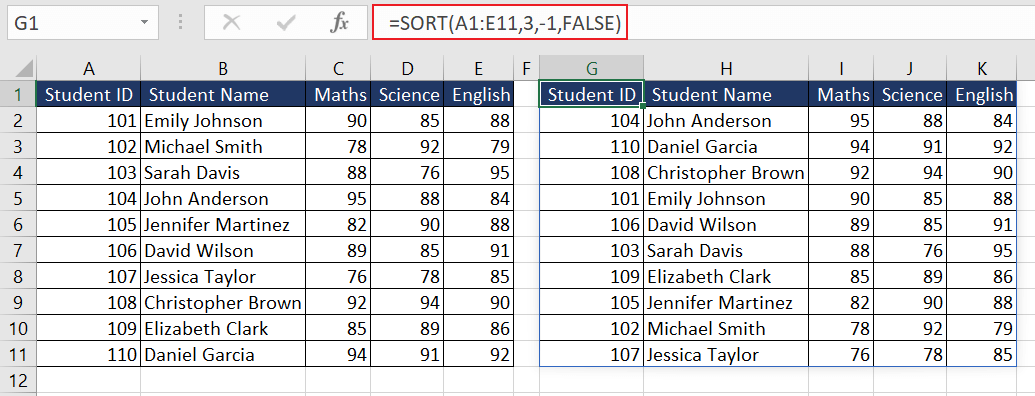
This is a classic use case of the SORT function. The goal is to rearrange the dataset as per marks scored in Maths. The student with the highest marks in Maths must be on top. The formula used will be as follows.

The formula aims to arrange the data in the array A1:E11 based on the marks obtained in maths, indicated by 3 indicating the column number, in descending order.

Now that we know who scored the highest marks in maths, let's move on to finding the lowest marks scored in science. We can again use the SORT function and change the input value of the sort_order argument to 1 indicating the ascending order.

As we wish to sort the dataset based on science marks (Column D), the formula used will be as follows.

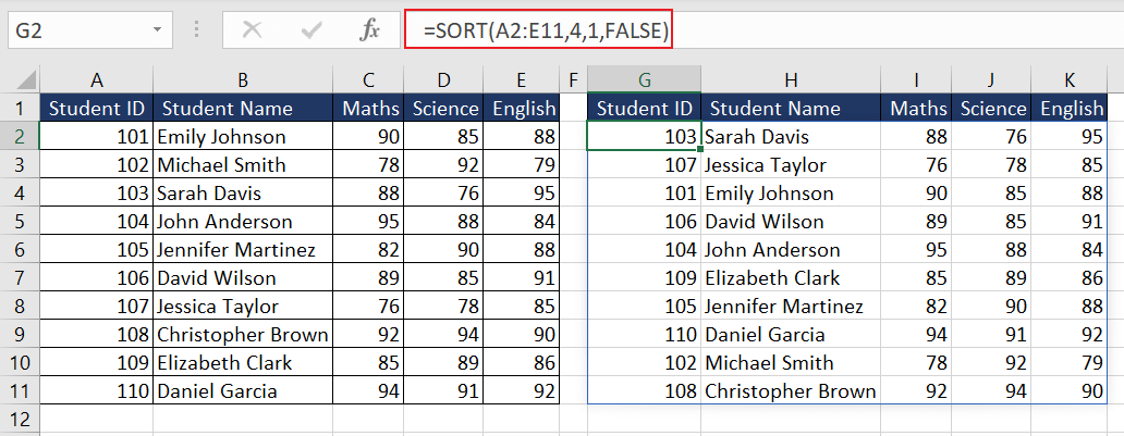
Now that we've learned how to rearrange a dataset using a single column, it's important to recognize that when working with extensive data sets, we often require multi-level sorting. In the next example, let's explore how to use the SORT function to rearrange the dataset by multiple columns in a different order.

Example 2 – Multi-level Sorting Using SORT Function

Imagine a scenario where you are managing a database of job applicants for a company's recruitment process. The database contains information about applicants, including their names, years of experience, and the department they are applying for.

Now, you want to sort the applicants first by their department in ascending order (alphabetical order) and then, within each department, sort them by years of experience in descending order (from most experienced to least experienced).

So, to ensure that we are including more than one column, we will use array constants for the input values of the sort_index and sort_order argument. The formula used will be as follows.

The first value in the array is 3 as column C contains the department they are applying for which will be sorted first. The sorting order for column C is defined in the third argument's array as 1, indicating ascending order. Next to be sorted is column B (given as 2 in the first array) – the years of experience, which is to be sorted in descending order (carried out by -1 in the third argument.

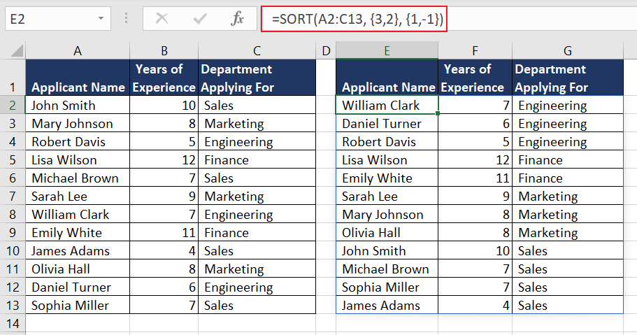
Now that you have the dataset sorted, you can forward the grouped applicants to the relevant teams.

Example 3 – Dynamic Sorting with SORT Function

Suppose you have downloaded some stock price data to analyze the daily prices of four stocks over a period. The dataset contains rows representing a different stock. Each entry is of the relevant stock's daily closing price.

We wish to reorder the dataset based on the Stock 2 prices in descending order. As the dataset will be sorted by column, we can set the input value of by_col to TRUE. The formula used will be as follows.

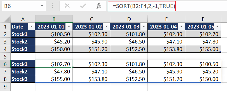
While the above solution successfully arranges the Stock2 data in descending order, it lacks the flexibility to accommodate additional data for future days. To ensure new data for the next days are automatically adjusted in a sorted manner, we can convert the dataset into Excel tables.

To do so, select the dataset (A2:F4) and click on 'Format as Table' on the Home tab. Let's name it 'stockprices'. Now the formula used will be as follows.

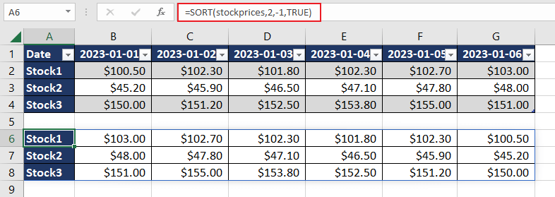
As we can see, when an additional column was added for the latest date, the returned dataset dynamically accommodates the new values. Therefore, a combination of the Excel table with the SORT function ensures that your table stays up to date as your dataset evolves.

Example 4 – Using SORT Function with FILTER Function

In this example, you have a large sales data which includes month-wise sales of a product along with the sales quantity and revenue. Your aim is to sort the products based on their total revenue along with the flexibility to choose different months to analyze.

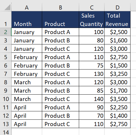
We can use the FILTER function to select data for a specific month and then sort the products within that month. Let's take cell G1 where the user can choose the month. The formula used will be as follows.

This will filter the dataset based on the condition that the "Month" column (Column A) should be equal to the value in cell G1. It selects rows where the "Month" matches the value in G1 and returns the corresponding data from columns A to D.

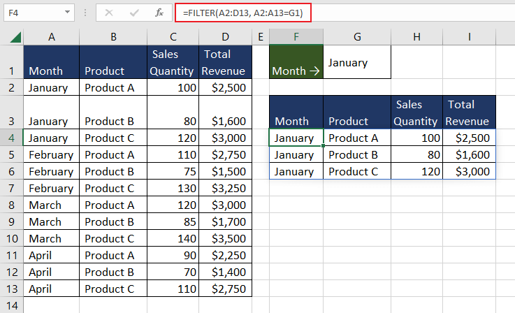
Now we have the data for the intended month, we will sort the data based on the fourth column, which is "Total Revenue," in descending order (-1). The final formula will be used as follows.

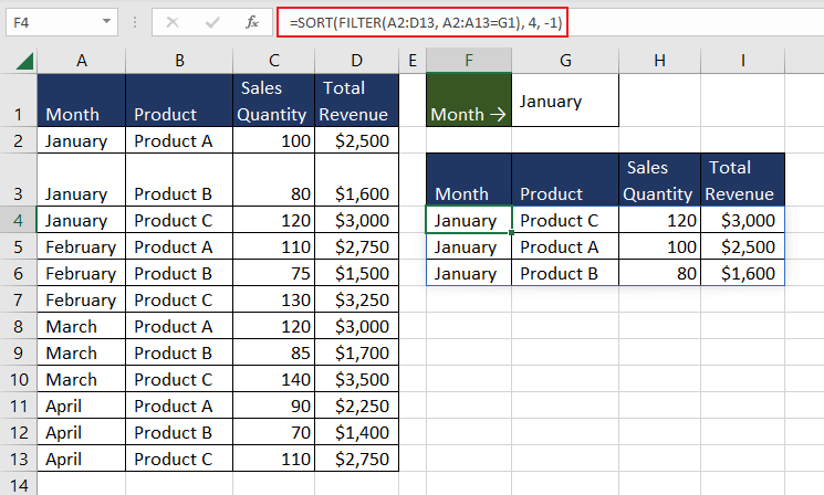
We now have the necessary month-wise data sorted in descending order based on revenue. The next day, what if you need to email the top 3 performing products as per the quantity sold? You can do so using the same SORT function combined with the INDEX function. Let's explore how to do that.

Example 4.1 – Using SORT Function with INDEX Function

As we want the top products based on quality sold, we will use the SORT function to reorder the data based on the values in the third column (column C) in descending order (-1). The SORT function returns a sorted array. The formula used will be as follows.

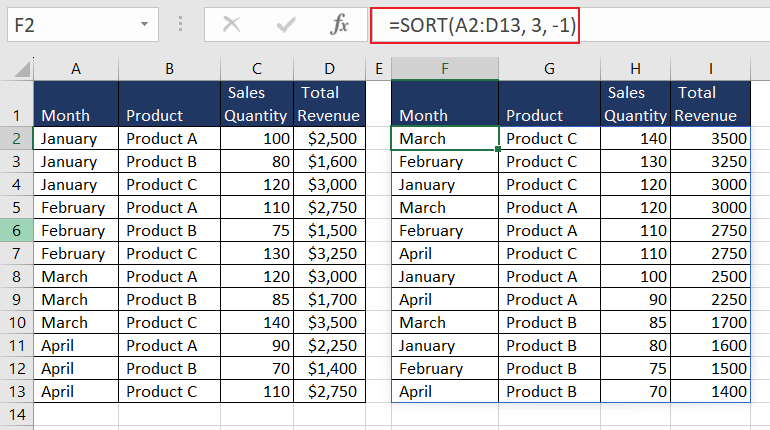
The next step is to use the INDEX function to retrieve the first 3 rows from the sorted dataset. Putting it all together, the formula used will be as follows.

Specifically, it extracts values from three rows (determined by SEQUENCE(3)) and three columns (determined by {2, 3, 4}) in that sorted range.

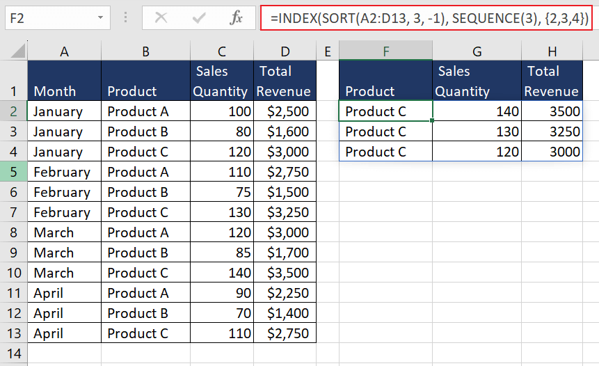
You can also use this logic to extract a sorted value from a specific position.

We now know that the SORT function in Excel is an indispensable tool for efficient data organization and analysis.

Practice to discover more applications of the said function and how you can include it in your daily work. While you improve your data manipulation skills with the SORT function, we will work on yet another Excel function to further add to your knowledge.