#NUM! Error In Excel – How To Fix

The #NUM! error is a frequent visitor on your worksheet. This can make you want to pull your hair out if you’ve used the output cell as a reference in another formula.

Looking for a fix? ExcelTrick has it for you.

What is a #NUM! Error in Excel?

#NUM! error occurs when you’ve entered a formula in your worksheet, but it can’t perform the calculation. For instance, say you’re trying to find square roots for a list of numbers. But there’s a negative value in the list. The formula will return a #NUM error for this value since it’s impossible to find the square root of a negative number.

But that’s not the only reason that can invite a #NUM! error into your worksheet. There are four possibilities that could be the reason for your perils. Fixing the error typically requires adjusting the values (no, it’s not mechanical, but an arithmetic error), and you’ll be set in no time.

Why Does it Appear?

So, why do #NUM! errors occur? Yes, as mentioned, there are four reasons. Let’s talk about them in a little more detail.

We already talked about the first reason in the previous section. If you’re trying to perform an impossible calculation, for instance, finding the square root of a negative number, you’ll get a #NUM! error.

The second reason could be that the output is too large or too small. The smallest and largest numbers that Excel can handle are -1*10^308 and 1*10^308, respectively. Excel displays any output outside this range as a #NUM! error.

The third reason could be that you’ve used an iterative formula that’s not finding a result. For instance, if you’re doing some capital budgeting and you’ve used the IRR formula in the process, and you see a #NUM! error, check the IRR formula. The IRR formula tries to calculate an answer that’s accurate down to 0.00001%. It tries to run about 20 iterations to find the answer. If it doesn’t, it returns the #NUM! error.

The fourth reason could be that you’ve entered an argument incorrectly in your function. For instance, think about the DATEDIF function. Things are all smooth sailing with this delightfully simple function, unless you mistakenly enter a start date that falls after the end date.

Sounds good? Perfect, let’s now try to look at how each of these reasons could play out on your worksheet and how to fix them with examples.

Examples

Following are some examples of when you’d see a #NUM! error.

1. Fixing #NUM! error when the calculation is impossible

When you’ve inadvertently asked Excel to perform an impossible calculation, you’ll see a #NUM! error. But the fix is, well, to make the calculation possible.

Let’s use the square root problem we discussed earlier. Say you’ve got some numbers in a list that you want a square root of, and you’ve applied the following formula to the numbers.

A negative number has sneaked into your list and caused a #NUM! error on your other spotless spreadsheet.

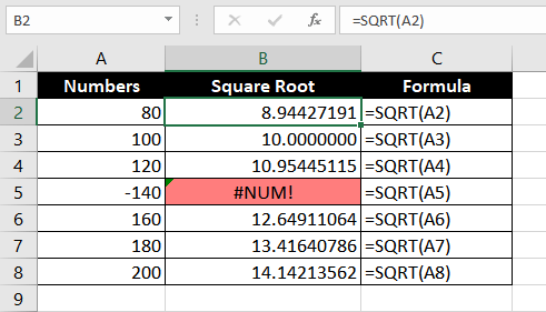
Once you’ve calmed yourself down from the panic of seeing the #NUM! error, think rationally. Since it’s impossible to find the square root of a negative number, you need to make it positive. The way to make it positive? The ABS function.

Here’s the formula you should use to fix the #NUM! error.

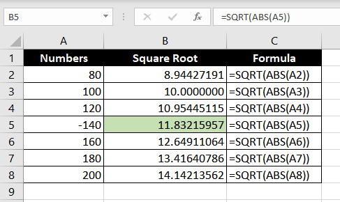
The ABS function converts the negative value into a positive one. When you enter a positive value into the SQRT function, everything should work fine. Easy-peasy, eh?

2. Fixing #NUM! error when the number is too large or small

The thing is… you can’t really fix this. If your output is too large or small for Excel, you’ll need to change your input to bring the output value within the acceptable range. For instance, say you’ve performed the following arithmetic operation in your Excel sheet:

Now, there’s no chance that Excel will be able to display this value, and will therefore return a #NUM! error. There’s no way to display the result, so you’ll need to change the output.

3. Fixing #NUM! error resulting from an iteration formula

Functions like IRR can sometimes also lead to a #NUM error. Such errors are mainly because of two reasons:

1. The specified Cash flow does not contain at least one negative and one positive value.
2. Formula can’t find a result.

Let's take the first case first.

In this example, we have listed down our cash flows within the range B2:B13. Now we will try to calculate the IRR using the formula below:

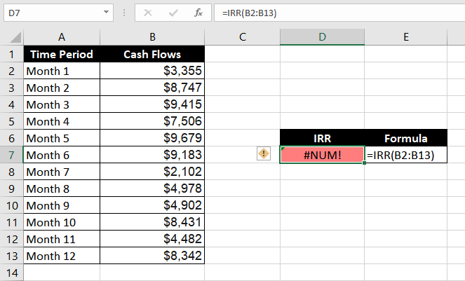
As we can see in the image above, excel returns a #NUM! error. The reason is pretty simple – the IRR function requires at least one negative value in the range as the initial cost of business.

So, in order to fix such an error, we can simply add our initial cost of business as a negative value to the cashflow range and the IRR function will display a valid result.

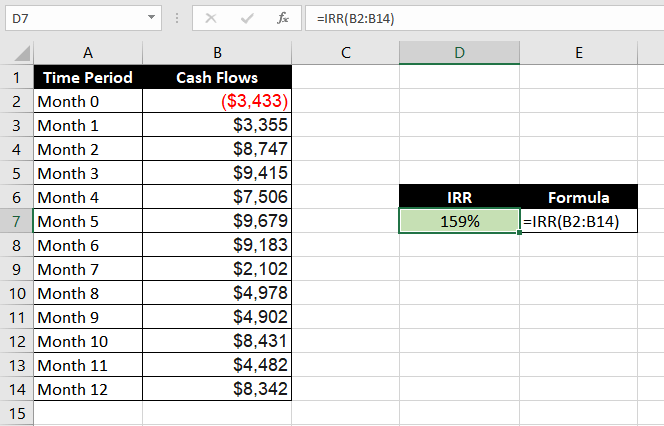
Another case, when the IRR function returns a #NUM error is when the function iterates and can’t find a result after several tries. We know that formulas like IRR and XIRR run several iterations to find an accurate answer.

However, Excel caps the number of iterations that these formulas go through so they’re not stuck in an infinite loop. When the formula maxes out the iterations without finding an answer, it returns a #NUM! error.

To overcome this, you have the option to increase the maximum number of iterations that Excel allows to get the result.

To increase the number of allowed iterations:

• Navigate to File > Options > Formulas to arrive at the window below
• Under the Calculation options group, check the Enable iterative calculation checkbox.

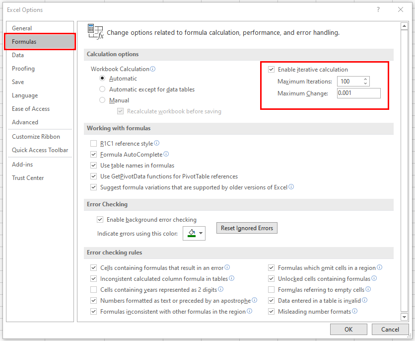
• In the Maximum Iterations textbox, enter the number of times you want Excel to perform iterations. Please note that – The higher the number of iterations, the more time and resources Excel might need to consume to display the result.

4. Fixing #NUM! error when you’ve entered an incorrect function argument

You can guess the fix before even looking through the example, can’t you? All you need to do is just enter the arguments correctly. Let’s look at how this will pan out practically.

Say you’ve got a few dates listed in two columns, and you’ve decided to find the differences between those dates. You remember reading our DATEDIF function tutorial, but you make a tiny mistake.

Understandable, right? If you read the DATEDIF tutorial carefully, you’ll see that Excel doesn’t show you the arguments you need to input as you type the formula, so this could be an easy mistake.

You use the start date as the end date and vice versa while applying the formula. So, you’ve incorrectly used the following formula.

The fix is simply to enter the arguments correctly into the formula, and that should eliminate the #NUM! error from your worksheet.

That’s all the ways you can deal with the #NUM! error whenever you find it on your worksheets. Child’s walk, right? While you champion eliminating #NUM! errors, we’ve got some more tutorials lined up for you. When you’re done, you know where to find us.