Let’s say you have an organization that makes hundreds of small transactions each day. You have several branches where the junior accountant punches in the numbers and dates into different software. It’s finally the end of the month, and you want to look at where you stand compared to the previous month.
This will require that you draw a gazillion charts, which is rather impossible to do unless you have a list of date-wise transactions. Since different branches may be using different programs, you will either need to import the data into an Excel file or type it in manually—you don’t have to be Einstein to make an instant choice here.
When you import data from databases, Excel may import those dates as text strings. The reason is, like Excel, not all programs store dates as serial numbers. When something is not a serial number, it’s not a date for Excel. This is why we are going to give you the rundown on some nifty formulas and methods that will help you create dates in your Excel worksheets.

How to Identify If Dates are Stored in Text?
When you try to use a certain list of dates with Excel tools like charts or PivotTables, they will fail to recognize data points as dates if they are stored as text. Although, there are several ways to just eyeball and determine if your list of dates are dates or text strings.
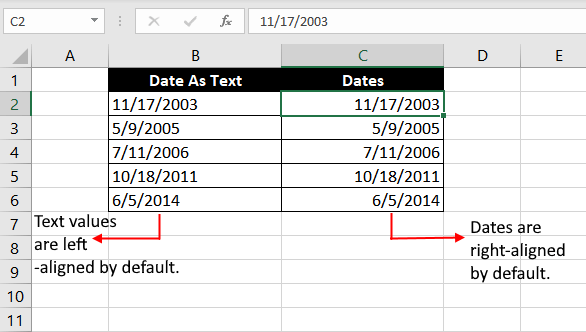
- Alignment
Excel right-aligns dates by default. If your list of dates is leaning on the left wall of the cell, it may make a light bulb go off. Those are not dates, they are text strings.
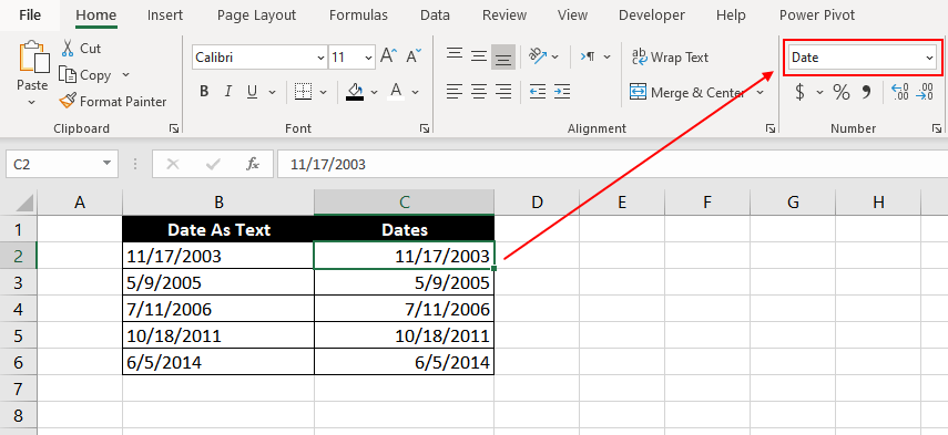
- Cell Format
The cell will be formatted as a “Date” in the Number Format box in Excel’s Home tab for data points that are recognized as dates by Excel.
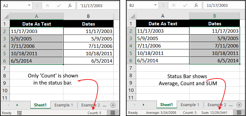
- Check the Status Bar
If you select the list of dates, you should see Average, Count, and SUM computed in the status bar, while you will see only Count if your dates are text strings.
3 Ways to Convert Dates Stored as Text
Let's see some of the ways to convert dates stored as text to a date value that Excel can recognize.
Method 1 – Using DATEVALUE and VALUE Functions
DATEVALUE function is a catalyst that changes a date in text format into a serial number that Excel will identify as a date.
The formula has a single argument where you will input the text string:
=DATEVALUE(A2)
Instead of adding a cell reference, you could also add a text string manually.
If you get a random five-digit number after using the formula, don’t panic. This is not a random number, this is the serial number that Excel recognizes as a date. To view it as a date, navigate to the Number group in Excel’s Home tab and change the cell’s format to Date — this should fix your output.
While DATEVALUE works perfectly well, the VALUE function goes a step further to include time in its return. Excel stores dates as a serial number, and time as a decimal value after that serial number. For example, if the serial number for December 25, 2001, is 37250, then 37250.5 will represent December 25, 2015, 12:00 PM, since 0.5 would mean half a day.
VALUE function’s syntax is similar to that of the DATEVALUE function:
=VALUE(A2)
Notice how the output for the first two rows returns 12:00 AM even though no time has been inserted for those dates under the DATES column. This is because Excel reads this as an integer (naturally, since there is no decimal value), and therefore assumes the time as 12:00 AM, i.e. 0 hours into the returned date.
In the last row, we have entered 15:00 (i.e. 3 PM) as time. Notice how the VALUE function returns a serial number with a decimal value. If you want to manually compute time using this decimal value, just multiply it with 24 (0.625 * 24 = 15).
Method 2 – Using SUBSTITUTE + VALUE/DATEVALUE Function
VALUE function is a catalyst that changes a date in text format into a serial number that Excel will identify as a date.
In our example, we will use the VALUE function, but the formula will work the same way even if you choose to use the DATEVALUE function. The only difference being that the DATEVALUE function will not return the time component if any is present in your cells.
Let’s set up an example: we have a list of dates with a delimiter other than a forward slash (/) or a dash (-). Excel is currently reading the elements of this list as a text string. There are two ways to convert these text strings into a date. We have the following list of dates:
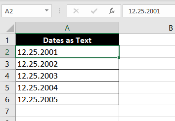
- First, we could use the Replace tool in Excel to replace the delimiter.
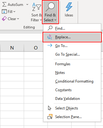
- Go to Home > Find & Select > Replace (Shortcut: Ctrl+H).
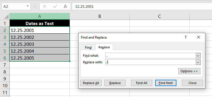
- In the Find and Replace dialog box, enter a full stop (.) in the Find what text box, and a forward slash (/) in the Replace with text box. Down below, hit the Replace All (i.e. leftmost) button.
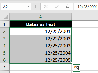
However, there is an easier way if you regularly populate your spreadsheet with new data — use a formula.
We know from our previous examples that the VALUE function is capable of converting text strings into a date. There is one caveat, though. Our text strings have a delimiter that keeps Excel from reading them as a date. So, we will need to supply a text string that has delimiters that Excel associates with a valid date.
Here’s the formula we will use:
=VALUE(SUBSTITUTE(A2, ".", "/"))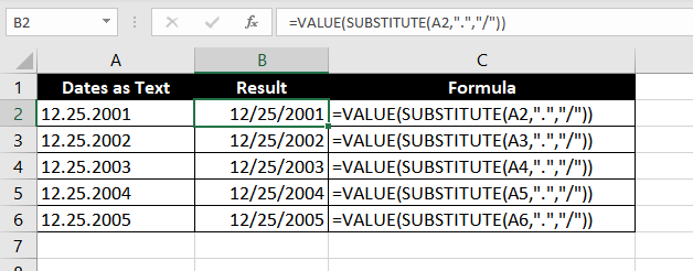
VALUE function does the same job here. It converts a text string into a date. We have nested a SUBSTITUTE function to deal with the delimiter issue. Had we directly referenced cell A2 inside the VALUE function, it would have returned a #VALUE! error since this text string cannot be recognized as a valid date in Excel.
All we need to do, then, is change the delimiter using the SUBSTITUTE function. Think of the SUBSTITUTE function as a formula for the Find & Replace tool we used in our previous example. It has 3 arguments: the first argument is a cell reference, the second argument is the character we want to replace, and the third argument is the character we want to replace with.
After executing the SUBSTITUTE function, our formula will look like this:
=VALUE("12/25/2001")This should give us our final output, an Excel-recognizable date — 12/25/2001.
Method 3 – Using Text to Columns tool for Complex Text Strings
Last year, you made a terrible decision of hiring a sloppy manager who didn’t bother to create separate columns for the weekday and date. This has led you to pull your hair while trying to analyze your sales data.
Fret not, we will work together and see this problem through.
The sloppy employee has made entries like so:
Tuesday, December 25, 2001.
To convert these strings to dates, we will use a two-step process. Step 1 involves using an Excel tool called “Text to Columns,” and Step 2 involves using the DATE and MONTH function.
Step 1:
- Select the list of text strings you wish to convert to dates.
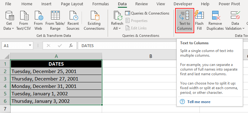
- Navigate to the Data Tools group under the Data tab and click on Text to Columns.
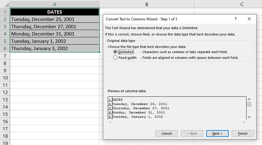
- Choose Delimited in the dialog box that opens, and click Next.
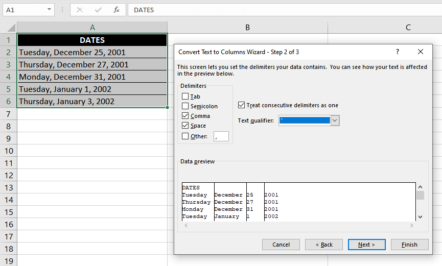
- On the next screen, you will choose the delimiters used in your text strings from the list. It is important to note that even space is considered a delimiter. Since our text strings have a space following the commas, we will check both delimiters on the list.
- At the bottom of the dialog box, you will see a preview of how the text strings will be split after you click Next.
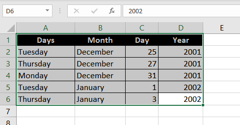
You have split the data, but there are still some miscellaneous things you need to run through. On the next screen, you will have the option to exclude any particular column from your output. For example, if the weekdays are irrelevant for you, exclude them by selecting the column (the column will turn black when selected), and choosing Do not import column (skip).
You may feel it is logical to choose Date under the Column data format list for the rest of the columns. However, remember that your text strings have been split into 3 components, and they cannot be recognized by Excel as a date. So, let them be formatted as General for now.
Finally, choose a destination where you want the return to be inserted, and click Finish.
Step 2:
We have our date split into three columns, and all we need to do now is bring them together and hand them over to Excel as a date. Although, there is still one loose end. Our month is a text string, while the DATE function needs a number.
To convert a month’s name to a number, we will nest the MONTH function inside the DATE function’s month argument. However, the MONTH function cannot work with just a text string, it needs a date so it can validly return the month number. We will circle back to this in a moment.
We will use this DATE formula:
=DATE(D2, MONTH(1&B2), C2)
If you are unfamiliar with the DATE function, take a quick tour of our DATE function tutorial.
The first and last arguments are just cell references to numbers that correspond to the year and date, respectively. So, what’s happening with the MONTH function?
Well, here’s what we are instructing the month function: Look at the value in D2 and give me the number from 1 to 12 for that month.
Had we only referenced the cell, the MONTH function could not have recognized the month. To remedy this, we concatenate a 1, which means it is now a date that the MONTH function can work with. 1 is just an arbitrary date, of course. You could have entered any number from 1 to 30/31 and it would still work.
So, we have now supplied the DATE function with all of its 3 arguments. This should give you a list of just the dates without the weekdays, and you can manipulate these dates in your worksheet as you see fit.
How and Why are Dates Stored as Numbers?
We know that Excel stores dates as serial numbers. Naturally, Excel does not just assign any random number to the dates; it follows a pattern. We will talk about this pattern in just a moment, but let’s first look at why Excel does this.
Why
There are several functions in Excel that manipulate the dates in the worksheet, including the DAYS, DATE, WORKDAY, DATEVALUE functions, among many others. These formulas need a standardized format that they can recognize as a date.
Consider that you are using the DAYS function, and have supplied two dates. You enter the end_date and the start_date and Excel computes the number of days to give you the output, i.e. the number of days between these dates.
In absence of serial numbers, Excel would have to use some alternate method to perform this computation. However, since Excel assigns a serial number, all it needs to do is subtract the two serial numbers and the resultant number will the number of days between these dates.
How
It is quite straightforward. Excel assigns ‘1’ to January 1, 1900. It adds 1 for each day from thereon. For example, January 2, 1900, will be assigned ‘2’.
January 1, 2021, is assigned 44197, which means 01/01/2021 occurs 44196 days after January 1, 1900.
This simplifies the computation and manipulation of dates to a great degree.
2 Ways to Convert Dates Stored as Numbers
We have some dates stored in our worksheet, but instead of being stored as dates, those cells have been formatted as General/Text/etc.
There are two ways we can convert these numbers to dates. Both instruct Excel to do the same thing, but in different ways.
Method 1: Format Cells Dialog Box
To convert the list of serial numbers to dates using this method:
- Select the cells containing the values.
- Navigate to the Number group under the Home tab in Excel.
- Select Short Date or Long Date from the dropdown menu. This should convert the numbers to dates. However, if you want a custom format for your dates, continue to the next step.
- Instead of opening the drop-down menu, click on the little arrow at the bottom-right of the Number group section. This should open up the Format Cells dialog box.
- Select Date on the list that appears at the left of the dialog box.
- You will see several date display formats listed in a box titled Type.
This will allow you to use a format of your choosing. However, if your desired format is not listed in the box, follow these steps:
- Instead of selecting Date from the list, select Custom. You will see several Custom formats listed in the box titled Type.
- If you want to create a format on your own, use the following codes:
| Code | Output |
|---|---|
| yyyy | Displays a 4-digit year: 1900-9999 |
| yy | Displays a 2-digit year: 00-99 |
| dddd | Displays weekdays: Sunday-Saturday |
| ddd | Displays 3-letter weekdays: Sun-Sat |
| dd | Displays the day component of the date, including 0: 01-31 |
| d | Displays the day component of the date, excluding 0: 1-31 |
| mmmmm | Displays the first letter of a month: J-D |
| mmmm | Displays the full month name: January-December |
| mmm | Displays the first three letters of a month: Jan-Dec |
| mm | Displays a number representing the month, including 0: 01-12 |
| m | Displays a number representing the month, excluding 0: 1-12 |
These codes will also come in handy while applying Method 2. Speaking of which…
Method 2: Using the TEXT Function
This time around, we will use the TEXT function instead of manually formatting the cells.
The formula we will use is:
=TEXT(A2, "mm/dd/yyyy")
The formula does a very simple thing. It looks at cell A2 and applies the format “mm/dd/yyyy” to the text string in that cell.
It is essentially the same as what we did with the Format Cells dialog box, but with a formula. If you want a different format, refer to the table of codes above and adjust your formula accordingly.
How to Convert an 8-digit Date to an Excel-Recognizable Date
This is not a valid 5-digit serial number that Excel can recognize as a date. Therefore, we cannot directly change the cell’s format to convert it into a date. We will need an alternative method that involves parsing the text string and pulling its various components together using several functions to get our final output.
Here is the formula we will use:
=DATE(LEFT(A2, 4), MID(A2, 5, 2), RIGHT(A2, 2))
The DATE function will help us assemble the different components of a date via its year, month, and day arguments. These arguments all have different functions that will relay the information to them.
The LEFT, MID, and RIGHT function pick out the relevant component from the text string and relay that number to the DATE function. In our example, the LEFT function looks inside cell A2 and relays the first 4 characters of the text string contained in cell A2 as a year argument in the DATE function.
You can also use this formula if you have different delimiters in the text string separating the year, month, and day components of the date. All you need to do is adjust the character count in the LEFT, MID, and RIGHT functions.
Fixing Text Dates with Two-Digit Years
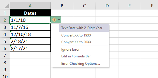
Unless you have entered a Custom format for any cell, a date that has a two-digit year will not sit well with Excel. Excel will add a green arrow at the top-left corner of each cell that has a date with a two-digit year.
To tackle this, hover your cursor over the cell. Doing this will bring up a drop-down button at the right of the cell with a yellow sign containing an exclamation mark. This sign tells you that there is an error, and you will see fixes (and other options) for the error in the dropdown menu.
The fixes will include two options, asking your preference regarding turning your dates into one that has a four-digit year. The first option will convert the year component into 19XX, the second will convert it to 20XX.
How to Enable/Disable Two-Digit Error Checking
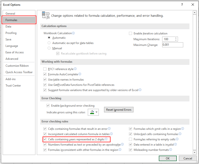
If you do not see the error warning, you may have disabled error checking. You can enable/disable error checking by navigating to File > Options > Formulas and checking/unchecking the box besides the option that reads Enable background error checking.
You will also see specific Error checking rules down below. To get a warning for two-digit years, make sure you have checked the box besides the option that reads Cells containing years represented as 2 digits.
This takes care of almost all methods of converting text or numbers to date in Excel. Several other formulas could be used as alternative methods since Excel has a giant pool of powerful formulas, but the ones we discussed should help you sail through almost any date-conversion-related issues.
Drill these techniques by practicing them. By the time they become second nature to you, we will have some more formulas for you to explore.


