Today you will learn how to sum filtered or visible cells in Excel. Our handy tools do so are a small handful of functions. Namely, the SUBTOTAL and AGGREGATE functions and a user-defined VBA function.
The need of the hour could be to group some data according to a particular attribute. Let’s say you want to see the sales figures of regions B and E from a dataset that includes figures from regions A to G. Or you may want to see batch sales greater than $200. Your choices are to filter the data or hide some rows or columns. Depending on the layout of your dataset, you may only have one option but either way, you will be left with filtered or visible cells.
The next step is to get the total of these visible figures.
Let’s get summing!

Problems with SUM Function
Calculate a total? Easy. Alt + H + U + S and you’re ready with the SUM function but that gives us a little trouble here. The problem with the SUM function is that it includes the cells excluded by hiding or filtering which renders the whole deal with hiding/filtering rather useless. Let us demonstrate.
In the table below, column H has been filtered to show post-tax totals greater than $200. If we select the filtered cells, the status bar shows us a sum of 903.56:
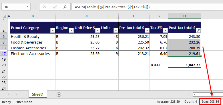
However, when we apply the SUM function to the filtered cells, we get a total of 1842.72:

What has happened here? Instead of taking just the filtered cells, the SUM function has taken all the cells between the first and last filtered cells. The formula has summed up the range H6:H17 which are 12 values instead of the 4 filtered values.
The same goes for hidden cells; since the SUM function takes a consecutive range (unless manually inputted with separate cells), hidden cells will also be included by the SUM function in counting the total.
Not an ideal situation this is. We obviously need a function here that can leave out filtered or hidden values and we certainly have it. Enter SUBTOTAL function.
Method #1 – Using SUBTOTAL Function
The SUBTOTAL function is used to calculate a subtotal in a dataset. The perk of this function is that it presents several options for calculating totals; sum, average, minimum value, maximum value, etc. It gives 2 options for calculating a sum; the first one works just like the SUM function and the other totals just the visible cells. That’s our target. Below we have the formula for summing the visible cells using the SUBTOTAL function:
=SUBTOTAL(109,H6:H17)The first argument is the function number. The number and its relevant functions are given while entering the SUBTOTAL function. You will find two options for sums; 9 and 109. Function number 9 is the option for the SUM function. Number 109 will also work for manually hidden cells.
Select 109 from the options so SUBTOTAL totals the values of the filtered cells.
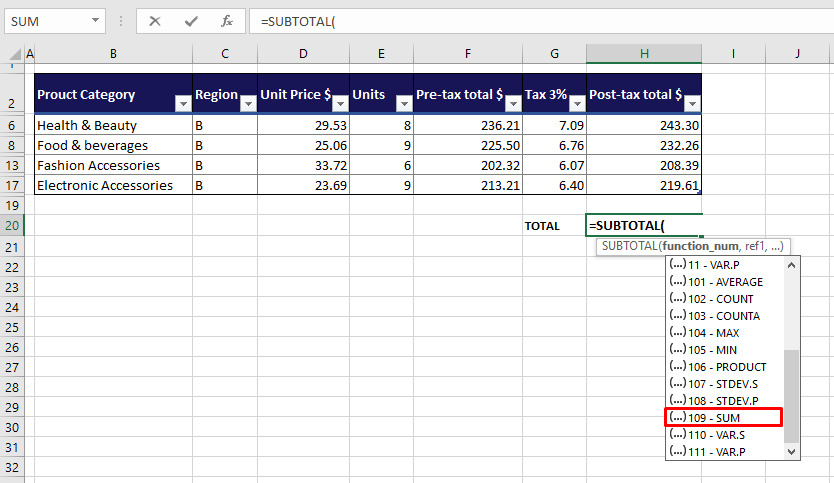
For the second argument, you can start referring the cells for summation. We have selected our visible cells which automatically becomes H6:H17 but thanks to the SUBTOTAL function, only the cells in display will be added.
We have our result:
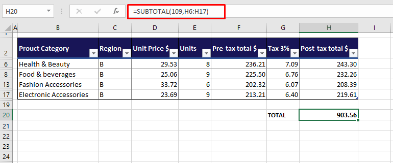
So the news now is that while this will work for hidden rows, it doesn’t work for hidden columns. If there is a hidden row along the range referred in the formula, their values will not be included in the result of the SUBTOTAL function. But if there is a hidden column, unfortunately those values will still make way into SUBTOTAL’s result.
We have another function that works like a copycat of the SUBTOTAL function for summing visible cells. Enter AGGREGATE function.
Method #2 – Using AGGREGATE Function
The AGGREGATE function returns an aggregate in a database. How is that any different from the SUBTOTAL function? There are few differences between the two and for returning a summation, they both work in a very similar way. Only that, in the AGGREGATE function, you can handpick what you want included or excluded from the total.
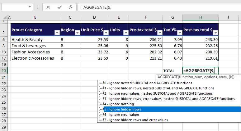
Let’s have a look at how the AGGREGATE function works for returning the sum of the visible cells. First, the formula we have used:
=AGGREGATE(9,5,H6:H17)Like the SUBTOTAL function, firstly comes the function number. Here, we have the number 9 for summation.
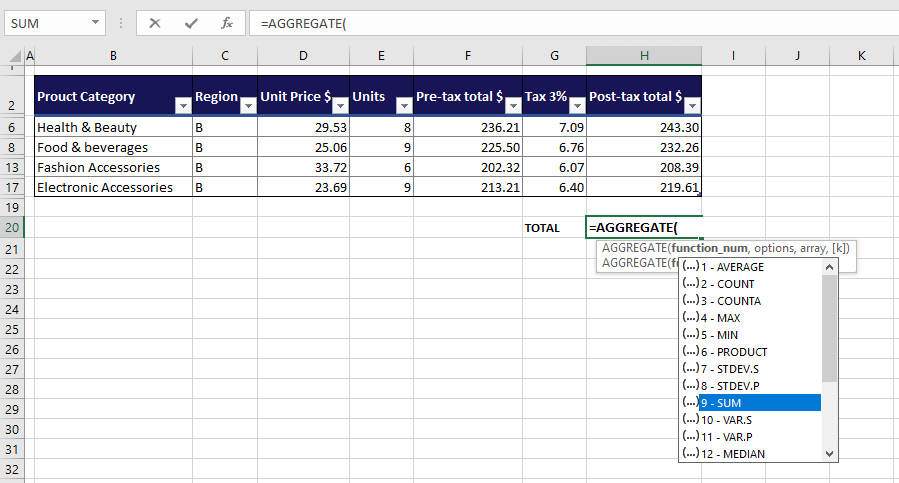
Next come the options for the values that are to be ignored from the aggregate. In our example, we need just the values in the filtered rows, making option 5 – ignore hidden rows a good fit.
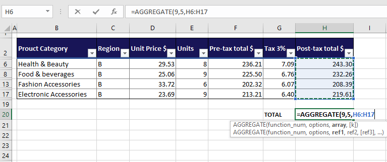
Now for the array. We have entered H6:H17.
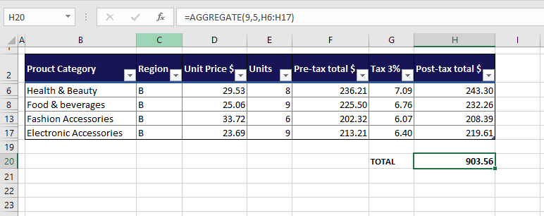
The AGGREGATE function has ignored the hidden rows to sum the values visible in the range H6:H17:
Notice how the options in the formula only mention hidden rows and not columns. Why? The AGGREGATE function also doesn’t work for hidden columns. Time to remedy that. Enter VBA function.
Method #3 – Using User-Defined VBA Function
In our final method, we will work with a user-defined function to get the sum of visible cells. No, we cannot just go creating functions in Excel at our whim, we will need VBA and a VBA code. The code will be used through VBA to create the function and then the function can be used on the worksheet, like all other functions.
Why go through the bother of creating a function? We had trouble leaving out hidden columns in the SUBTOTAL and AGGREGATE functions. In this VBA function we speak of, we can have the function leave out hidden rows as well as columns. Win-win all over.
Here’s how we’re going to use a user-defined function in VBA for the summation of visible cells:
- Press the Alt + F11 keys to launch the VB Or, if you have the Developer tab added, you can go to the tab’s Code group and click on the Visual Basic button.
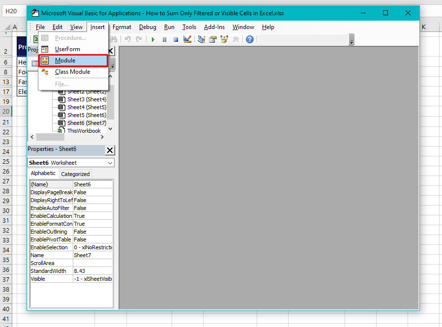
- Once the VB editor is open, click on the Insert tab and select Module from the list. You will be redirected to a Module window.
- In the Module window, copy and paste the code below to add the function:
Function SumVisible(WorkRng As Range) As Double
Dim rng As Range
Dim total As Double
For Each rng In WorkRng
 If rng.Rows.Hidden = False And rng.Columns.Hidden = False Then
 total = total + rng.Value
 End If
Next
SumVisible = total
End Function
A function will be created with the name “SumVisible” to calculate the total of the selected cells that are visible in the dataset, ignoring values in hidden rows and columns.
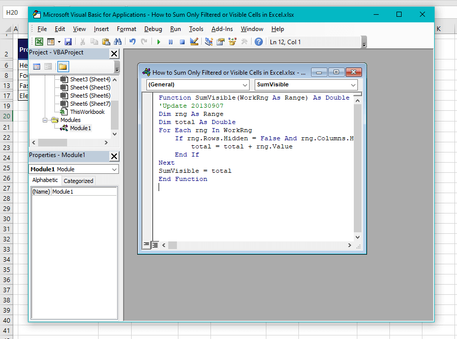
- Close the VB
- In the cell where you want the total, enter the following formula:
=SumVisible(H6:H17)You only need to enter the created function’s name and the range. The function will sum the values in the range and return the total:
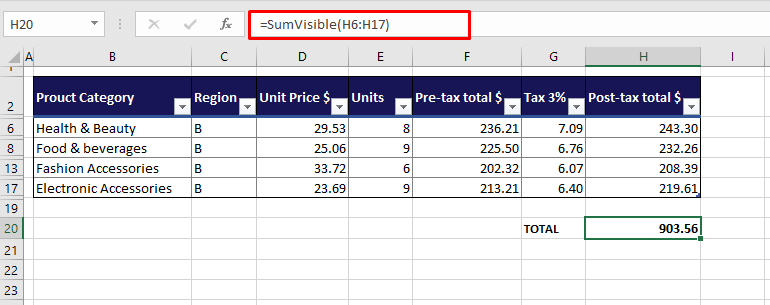
Note: The values in hidden rows and columns will be left out from the calculation. Do note however that once the formula has been entered, after that if you are to hide a row, the result will adjust to exclude the value hidden. But if you hide a column, you will have to recalculate the formula as it will not automatically adjust for the hidden column’s values.
You can simply recalculate by selecting the cell with the formula, going into cell edit mode, and pressing the Enter key.
To sum it up, those were some easy ways to sum only filtered or visible cells in Excel. Mostly for datasets like our case example, you’ll be good using the SUBTOTAL or AGGREGATE function which will ignore hidden rows. For getting hidden columns ignored, you will need to create a VBA function. There, that’s the whole story. We’ll be back with more Excel stories and fairytales to combat your Excel villains!


